Buletin Ilmiah Sarjana Teknik Elektro ISSN: 2685-9572
Fuzzy A* for optimum Path Planning in a Large Maze
Gregorius Airlangga
Information Systems Study Program, Universitas Katolik Indonesia Atma Jaya, Jakarta, Indonesia
ARTICLE INFORMATION |
| ABSTRACT |
Article History: Submitted 19 October 2023 Revised 28 November 2023 Accepted 30 November 2023 |
| 
Traditional A* path planning, while guaranteeing the shortest path with an admissible heuristic, often employs conservative heuristic functions that neglect potential obstacles and map inaccuracies. This can lead to inefficient searches and increased memory usage in complex environments. To address this, machine learning methods have been explored to predict cost functions, reducing memory load while maintaining optimal solutions. However, these require extensive data collection and struggle in novel, intricate environments. We propose the Fuzzy A* algorithm, an enhancement of the classic A* method, incorporating a new determinant variable to adjust heuristic cost calculations. This adjustment modulates the scope of scanned vertices during searches, optimizing memory usage and computational efficiency. In our approach, unlike traditional A* heuristics that overlook environmental complexities, the Fuzzy A* employs a dynamic heuristic function. This function, leveraging fuzzy logic principles, adapts to varying levels of environmental complexity, allowing a more nuanced estimation of the path cost that considers potential obstructions and route feasibility. This adaptability contrasts with standard machine learning-based solutions, which, while effective in known environments, often falter in unfamiliar or highly complex settings due to their reliance on pre-existing datasets. Our experimental framework involved 100 maze-solving trials in diverse maze configurations, ranging from simple to highly intricate layouts, to evaluate the effectiveness of Fuzzy A*. We employed specific metrics such as path length, computational time, and memory usage for a comprehensive assessment. The results showcased that Fuzzy A* consistently found the shortest paths (99.96% success rate) and significantly reduced memory usage by 67% and 59% compared to Breadth-First-Search (BFS) and traditional A*, respectively. These findings underline the effectiveness of our modified heuristic approach in diverse and challenging environments, highlighting its potential for real-world pathfinding applications. |
Keywords: Fuzzy; A*; Path Planning; Maze; Optimization |
Corresponding Author: Gregorius Airlangga, Universitas Katolik Indonesia Atma Jaya, Jakarta, Indonesia. Email: gregorius.airlangga@atmajaya.ac.id |
This work is licensed under a Creative Commons Attribution-Share Alike 4.0 
|
Document Citation: G. Airlangga, “Fuzzy A* for optimum Path Planning in a Large Maze,” Buletin Ilmiah Sarjana Teknik Elektro, vol. 5, no. 4, pp. 455-466, 2023, DOI: 10.12928/biste.v5i4.9394. |
- INTRODUCTION
Path planning is essential for an autonomous agent to proceed from its starting point to its destination while avoiding obstacles and achieving its goals [1][2]. Generally speaking, the goals are the shortest path and optimal memory consumption [3]-[5]. This task becomes increasingly challenging in complex [6]-[9] and vast environments, often categorized as Maze-Like or Labyrinth challenges [10]-[14]. Several methods, including Djiskstra’s, Breath-First Search, Depth First Search, Greedy Algorithm, Best First Search, and A*, have been utilized to solve the problem. However, despite creating an optimal path, Djikstra’s and Breath-First search compromise memory efficiency due to the extensive exploring characteristics of traversing each nearby vertex until the goal is reached [15]-[19]. In contrast, algorithms such as Best First Search, Depth First Search, and Greedy algorithm can effectively guarantee path completeness; but, they may miss major path optimality with dead-end paths by constructing paths that are typically lengthy and circular [20]. A* algorithm is the most effective method for achieving a balance between optimal path and memory consumption. In many instances, the algorithm can guarantee not only completeness, but also memory efficiency and global optimality [21].
The A* algorithm estimates costs using a heuristic function. The heuristic function must have admissible heuristic characteristics that do not exaggerate the cost in the searching space in order to guarantee a global optimal solution. Although admissible heuristic functions effectively generate an optimal path, the heuristic functions are typically constructed conservatively to avoid overestimating the significance of obstacles, objective directions, and infeasible regions on the map. The characteristic causes the calculation time and visited vertex count to explode, particularly when the environment contains numerous local dead-ends [22][23]. For this circumstance, the back-track technique could be relocated far from the last dead-end point that requires calculating an adjacent collision-free position. Even if the computation time increases, the technique can still ensure the optimal global answer.
| 
| (1) |
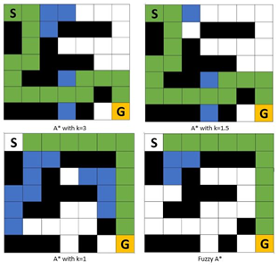
In order to reduce memory consumption, the heuristic function can be defined flexibly, since the searching process can result in a stronger force to locate a path more quickly by not exploring many vertices. The search can be undertaken using the heuristic inflation illustrated in equation (1). The first equation clearly demonstrated that the cost of a successor vertex vj is determined by the true cost and heuristic function times constant k values. The effect of k value is to exaggerate the heuristic value. By using the formula, the produced path can have cost result not greater than k times than the cost of the global optimal paths. This condition is well-known as bounded suboptimality [24]. The effect of the k value is visualized on the Figure 1.

Figure 1. The effect of the k value
Based on the Figure 1, when k > 1 times, the number of visited vertex can be reduced while sacrifice the optimal path. Therefore, by observing those characteristics, the optimal heuristic cost can be achieved by combining other approaches that predicting the cost to minimizing searching space while guarantees the optimal path. Several researchers have initiated the research by using machine learning approaches such as [25]-[29]. However, data-driven approach is unstable, slow to converge and susceptible to poor local optima. In addition, the approach is dependent on the data preparation and hyper parameter tuning. Even if, the heuristics can be predicted optimally, however due to the black box characteristics, the method is not adaptable to be analyzed for further situations, therefore it cannot always guarantee the global optimum [30].
In this research, we present an innovative way for adjusting the heuristic function of the original A* algorithm by altering the equation one. We suggest a variable parameter known as the Strength Direction Parameter, which is governed by a Fuzzy-Logic prediction approach. Our technique differs from existing path planning approaches that independently employ Fuzzy methods and A* methods. We merge these methods into a single algorithm to determine the shortest path. At each iteration, the fuzzy-controller decides the Strength Direction parameter for the A* mechanism by examining the present state of the current vertexx candidate. The fuzzy-controller employs the number of visited vertices, the number of obstacles, and the current distance to control the strength direction parameters. The parameter itself plays a crucial function in determining the candidate visited vertex at each iteration towards goals. In Section 2, we provide a complete explanation of the suggested technique. In Section 3, we present the theoretical analysis by examining the algorithm and its effectiveness. In addition, experimental analysis is presented in Section 4, and the conclusion and future work are explored in Section 5.
- METHOD
In this part, there are five subsections that explain the proposed Fuzzy A* approach. First, we discuss the formulation of the problem in a vast maze setting, followed by the rationale for modified A*. In the third subsection, we discuss the fundamental concept underlying the modified A* method with the Strength Direction parameter. In the latter two subsections, we describe the fuzzy logic behind the suggested method and its algorithm.
- Problem Formulation
In this study, we examine the graph path planning problem  where
where  is the set of feasible vertices and
  is the set of edges connecting pairs of vertices in , whose costs are
  . Typically, each viable vertex corresponds to an obstacle free map or environment configuration. A feasible path from
  to
to  can be represented as a sequence of vertices in
  , where
  and
and  , while there exist all the edges connecting adjacent vertices,
  for
for  }. The cost of a path is the total of the costs of its edges,
  for all feasible paths,
  with the same boundary condition, the total cost of the path can be defined as
  .
.
The difficulty occurs when the agent is entrusted with determining the ideal path  in a vast environment, if pathways have a large number of obstacles and dead-end vertices, then they are deemed to be obstructed and dead-end. To ensure global optimality, this may result in the evaluation or exploration of all potential vertices. The searching procedures may be exponentially proportional to the environment's dimension count. On the other hand, despite the fact that the admissible heuristic
  can ensure the global optimal path, the heuristic function is typically constructed conservatively to avoid overestimating the value of barriers, goal directions, and infeasible regions in the map. Additionally, the heuristic depends on the environment's characteristics. In order to reduce such evaluations, several modifications of the graph search algorithm have been designed to guarantee the existence of a bounded suboptimal path whose cost does not exceed
  times that of the optimal path. In this paper, the suggested Fuzzy A* algorithm is designed to reduce computation burden by altering extra Strength Direction parameters in the heuristic function used in calculation. At each iteration, a dynamic and intelligent decision is made to provide the ideal path while minimizing the number of expanding vertices.
- Motivation of Fuzzy
Our method is primarily motivated by the original characteristics. Consider an agent on a Graph with an order to traverse from the start point to the goal location  . The movement is governed by two primary constraints: the shortest path must be found, and the searching process must be as memory-efficient and quick as possible.
As previously noted, with admissible heuristic might be seen as a solution for achieving the aim. Even if the suitable heuristic function can lead to the ideal path and reduce memory consumption, memory consumption and searching process time still take a significant percentage in many circumstances, particularly when the environment expands, and the number of barriers increases. To guarantee the optimal path, a heuristic function of  must has admissible property [10], hence, the heuristic value is never greater than the actual cost of reaching the goal from
  . By enhancing the heuristics with a constant value
  for
for  , the algorithm results in significantly fewer state expansions and, as a result, speedier searches. Using this approach, however, can break the admissibility property; as a result, an optimal solution is no longer guaranteed.
Because numerous preceding methods, like weighted  , and
, and  , inflate the heuristics by a predefined cost at each iteration until the goal is accomplished, the searching process can overestimate the vertex value if the true cost of the shortest path is not meticulously assessed. In contrast to these methods, we adjust the heuristic function at each iteration using the Strength Direction Parameter (SDP). The value change may be either moderate or significant. If the direction is weak, the cost of the visited vertex will be increased by the value of the weak direction, and vice versa. In addition, the Fuzzy prediction model can provide a smooth value by considering three input variables, such as the number of barriers, the number of visited vertices, and the current distance from the current vertex position to the objective.
- Modified Heuristics
Initially, accepts as input a heuristic  which must be consistent, that is
  For any successor vertex
  of if
of if  and
and  if
if  . Here
  represents the cost of an edge from to and must be positive, in many cases, the default of additional cost is defined as one since each adjacent vertex considered to be closely spaced. Consistency, in its turn, guarantees that the heuristic is admissible: is never larger than the true cost of reaching the goal from . In our approach, we replace the constant additional cost that assigned at each iteration into Strength Direction Parameter (SDP), where
  and
and  set of Directions.
The dependent variable  in the equation (2) is modified at each iteration by a Fuzzy prediction model that relates the position of each succeeding vertex to the position of the target vertex. The details of Fuzzy prediction model are explained in Section Fuzzy Prediction Model. Once value of the equation (3) has been obtained. If the successor vertex satisfies the condition where the successor vertex's real cost path value is greater than the total of the current vertex and default cost value, then the true cost path of is updated by adding to
  and . Finally, the cost function in equation (4) will be adjusted by including the improved heuristics.
The generated updated cost compares more smoothly than the default cost because, at each iteration, the searching space can prevent false directions by overestimating the linked successor vertex that moves in incorrect directions. In contrast, the true direction will have a low-cost value, which will lead to the dominant election state which has the true direction at each iteration. This is because the smallest value  should be chosen as a new candidate at each iteration until
  is located.
- Fuzzy Prediction Model
This study expands upon the functional method by applying it to a fuzzy prediction model for path planning. Numerous variables affect the value of the decision path, making it impossible to predict it with precision. The proposed Fuzzy A* method generates a fuzzy set of trapezoidal shape that indicates both the representative value (modal value) and the support interval of the predicted value. The input variables for this model are the number of barriers, the number of visited grids, and the distance between the agent’s present position and the objective. The output variables weakPowerDirection and strongPowerDirection are examples. We use the fuzzy prediction model of Shimakawa and Murakami [16] to automatically generate weakPowerDirection and strongPowerDirection values. The rules used in this investigation are derived from the equation (5).
| 
| (5) |

|
Where  represent input variables and
  and
and  represent outcome variables. Moreover,
  and
and  are fuzzy set representations. The
  position parameters and
  position parameters define the fuzzy sets
  , and . Each fuzzy set's membership function shape is constructed using the position and height parameters. The position parameter represents a set of
  -axis values that specify the form or width of the membership function. Alternatively, the height parameter represents the height of the membership function at a certain position parameter. The fuzzy set of , and is therefore characterized by the membership function
  , as indicated in equation (6).
| 
| (6) |

|
In this work, we use trapezoidal membership function. Equation (7) shows the formula. This function depends upon four position parameters  and a height parameter
  .
.
| 
| (7) |
Using equation (6), we can define R's fuzzy relationship. Based on all input variables, a fuzzy relation function will be utilized to reason. Moreover, the fuzzy relation function itself is a membership function of  that maps input
  into and where denoted as
  and
and  [17]. The
  membership
  depends on weighted averages of each position parameters and weighted sum of each height parameters. In addition, using max-min rule to find the relationship the membership function will be defined as equation (8).
Where  are the antecedent part membership functions.
  as presented in equation (12) reflects the compatibility levels for each fuzzy rule's antecedent portion.
  and
and  determine the position and height parameters between the fuzzy rules using equations 10 and 11 respectively. The fuzzy relation is defined using membership function which contains parameter
  and
and  * the height of the membership function also become zero. For the case in which exceeds 1, equation eight must limit the height of the membership function to 1.
In the case of high overlapping fuzzy sets  of the antecedent part, the value of is likely to exceed 1, leading to a subnormal result. Consequently, this might be viewed as a restriction of the approach, as the relation will not be able to differentiate between circumstances that overlap. In other words, all membership levels would equal the maximum value of 1….0.
- Fuzzy
The Fuzzy A* algorithm employs three primary functions: the Heuristic Function, the Main Fuzzy function, and the FindDirection function. In our proposed strategy, the additional cost between adjacent vertices is separated into two groups. First, we create the default cost value, which is set to one, and the Strength Direction Parameter, which has a dynamic value derived from a fuzzy inference function that considers three input variables, including NumberOfObstacles, CurrentDistance, and VisitedGridCounter. The input variables will then generate two output variables, including weakPowerDirection and strongPowerDirection. The specifics of the fuzzy inference system have already been described in Section 2.4.
Since the heuristic function must be admissible to guarantee the optimal path, the heuristic value is never larger than the true cost of reaching the goal from . By improving the heuristics using a constant value  for , The technique yields significantly fewer state expansions and, thus, quicker searches. However, applying this approach can violate the admissibility property, and as a result, the optimality of a solution cannot be guaranteed. Our proposed method is inspired by these properties, in which adjusting the appropriate value at each iteration leads to the reduction of the number of the visited vertices while maintaining the property of admissibility.
The dynamic cost value will be initiated as weakPowerDirection if the direction from the current state to goal is indicating the true direction, then weakPowerDirection  and otherwise initiated as strongPowerDirection if false direction state assigned in the successor vertex , thus strongPowerDirection
  . weakPowerDirection has a membership values between 0…..0.001 and strongPowerDirection has membership values between 0-100. Based on the present heuristic function, using the weakPowerDirection can inflate a modest value. The heuristic value of the successor vertex can be evaluated with attention as opposed to a hasty pursuit of the goal. This approach enables the searching process to maintain the optimal path location by decreasing cost while remaining vigilant, particularly when the future child vertex contains numerous barriers with dead-end positions. In addition, by incorporating a big value between 0 and 100 into the false direction, we assign a high value wo the candidate vertex that indicates a penalty if the vertex is classified as a false direction, thus enhancing the visited vertex, and maybe containing numerous barriers.
The pseudocode of the Fuzzy A* approach in Algorithm 1, Algorithm 2, and Algorithm 3 are merely the simple formula of the Euclidean Distance function, which is of ten employed as a Heuristic Function on 4-direction, 2-grid maps. In our experiment, we apply the formula to execute the and Fuzry programs. The Fuzzy method maintains two functions from states with real numbers: the cost of the currently found path from the start vertex to current ( ) and it is assumed to be 0 if no path to has been found yet, and  is an estimate of the total distance from start to goal going through . The Fuzzy method additionally maintains a priority Min Heap, OPEN_HEAP, of vertices that it indents to expand. The OPEN_HEAP
  is ordered by from least to maximum, such that the Furry algorithm always extends the vertex that looks to be on the shortest path from start to goal.
Figure 2 depicts the pseudo code of the very important module in Fuzzy A* approach, which is the formula for determining the direction from the present vertex to the target. Assume there are four direction vertices that go to the goal position: [north, south, left, and right]. If the current vertex position is positioned to the north-left of the target position, then the function returns the values  . The returned value will be used to determine whether weakPowerDirection or strongPowerDirection will add cost to the successor vertex.
1: Input: startNode, goalNode; 2: Result: distance; 3: distance = √((startNode.x - goalNode.x)² + (startNode.y - goalNode.y)²); |
Algorithm 1. Euclidean distance
1: g(s_start) ← 0; 2: OPEN_HEAP ← ∅; 3: PARENT_SET ← ∅; 4: VISITED_NODE ← ∅; 5: H ← Euclidean(s_start, s_goal); 6: f(s_start) ← H; 7: insert s_start into OPEN_HEAP; 8: visitedNodeCounter ← 0; 9: obstaclesCounter ← 0; 10: obstaclesChecked ← ∅; 11: numberOfPossibleDirections ← 4; 12: strengthDirection ← zeros(numberOfPossibleDirections, 1); 13: fuzzyKnowledge ← callKnowledge(); 14: default_cost ← -1; 15: while f(s_goal) > min OPEN_HEAP(f(s)) do 16: remove s with the smallest f_value from OPEN_HEAP; 17: if s not in VISITED_NODE and s not obstacle then 18: insert s into VISITED_NODE with state(s) ≠ obstacle; 19: else 20: update s from VISITED_NODE with state(s) = obstacle; 21: end if 22: visitedNodeCounter++; 23: currentDistance ← Euclidean(s_current, s_goal); | 24: for each successors s' do 25: if isEmpty(obstaclesChecked(s')) then 26: insert s' into obstaclesChecked; 27: obstaclesCounter++; 28: end if 29: if s' was not visited before and not the obstacle then 30: f(s') ← ∞; 31: g(s') ← ∞; 32: end if 33: weakPowerDirection, strongPowerDirection ← fuzzyInference(); 34: Directions ← findDirection(s_current, s_goal); 35: for all d in D do 36: if d == 1 then 37: strengthDirection(d) ← weakPowerDirection; // β ∈ (0,...,0.01) 38: else 39: strengthDirection(d) ← strongPowerDirection; // β ∈ (0,...,100) 40: end if 41: end for 42: if g(s') > g(s) + default_cost then 43: g(s') ← g(s) + strengthDirection(d); 44: f(s') ← g(s') + Euclidean(s_current, s_goal); 45: insert PARENT_SET with parent=s and child=s'; 46: insert s' into OPEN_HEAP with f(s'); 47: end if 48: end for 49: end while |
Algorithm 2. Fuzzy A* method
1: Input: startNode, goalNode, numberOfPossibleDirections; 2: Result: Directions; 3: begin 4: difference_y ← startNode.y - goalNode.y; 5: difference_x ← startNode.x - goalNode.x; 6: Directions ← zeros(numberOfPossibleDirections, 1); 7: if difference_x > 0 then 8: Directions(x_axis) ← 1; 9: end if 10: if difference_y > 0 then 11: Directions(y_axis) ← 1; 12: end if 13: end |
Algorithm 3. Find direction method
- THEORETICAL ANALYSIS
In this part, some of the theoretical features of the proposed Fuzzy approach is discussed. In the theorems we used *(v) to represent the optimal cost from vertex  to . There are three accompanying notes for this section. First, we have just included the line codes stated in this section in Algorithm 2. Second, we assume a greedy algorithm as a comparison by establishing a greedy route from
  to
to  , and at each vertex
  we choose a vertex
 until
until  . Finally, we define the recurrence visited vertex (RVV) as the condition in which the visited vertex is reused as the current vertex for path calculation, thereby reducing the total number of candidate successor vertex on the subsequent iteration because the previously chosen successor vertex will be defined as an obstacle.
Theorem 1: When function of insert of successor vertex into collections of OPEN_HEAP with  returns, for any vertex
  with
with  will have the value
  and the loop will end.
Proof: The function of can only change on line 43 if the condition  default_cost is met; afterwards, the function is utilized to determine the value of . When
  is reached, the statement on line 46 will add the vertex(v) to OPEN_HEAP. Therefore, on the following iteration, the value of
  will change from
  to
to  , and when the vertex are reached, the iteration will end and the condition
  will be satisfied.
Theorem 2: For each pair of vertices  and
and  , the value of
  weakPowerDirection
  strong PowerDirection and the value of from weak PowerDirection
  from strongPowerDirection.
Proof: Line 33 determines the values of weakPowerDirection and strongPowerDirection for each iteration. Before further assignment to line 37, line 39, and line 43 correspondingly. The implementation of Fuzzy knowledge on line 13 generates weakPowerDirection, which has a modest value between  and strongPowerDirection
  . The validity of the theorem may thus be demonstrated.
Lemma 3: PARENT SET values are limited to a maximum of numberOfPossible Directions pairs between parent and child vertices.
Proof: Given a vertex and a value of four for number  . Possible Directions: four possible directions will be considered. The vertex are next to vertex with free collision obstacles. Consequently, according to the line 24, every
  on the successor vertex can be regarded as a possible vertex. Additionally, the syntax on line 45 will push the pair information between parent vertex and four free collision obstacles vertex as offspring vertices into the PARENT_SET.
Theorem 4: Recurrence visited vertex (RVV) can occur no more than  times, where is calculated from the equation (13) and representing several maximum revisited vertex occurs,
  is the number of alternative directions of the current vertex and
  denotes the number of possible obstacles. Before and after a RVV, the value of successor vertex
  is always changed and must fulfill
  .
.
| 
| (13) |
Proof: When RVV cocurs, the selected vertex will be determined by the smallest value of OPEN_HEAP on line 16 where  , when vertex is re-selected as the current vertex, the successor vertex will no longer be . In addition, the strong PowerDirection parameter will update all potential values with the increment value of numberOfObstacles (the previous selected successor vertex will be considered obstacles).
Theorem 5: At line 1, the cost of vertex in start position is always zero  and for another vertex
  is met.
Proof: From the first line, it is evident that when  , the remaining values are not zero. The only location where values change is on line 43. If is modified, the c-values of its descendants will drop. The test at line 42 verifies this and, if required, changes the -values. Since all default cost are constant and positive,
  can never change and is consequently always 0.
Theorem 6: In the worst-case situation, where several RVV occur, the cost of the suggested Fuzzy technique will exceed that of the greedy path 
 .
.
Proof: As stated in Theorem 4, the values of will differ from prior values. In this condition, the candidate for the next vertex can be derived from  strongPowerDirection, as the knowledge-kased properties provide much greater value than the default cost considered by the greedy path algorithm; consequently, the total cost from to will always be greater than the total cost generated by the greedy path algorithm.
Theorem 7: In the best-case situation, when RVV does not occur, the proposed Fuzzy technique will be considerably less expensive than the greedy path. 

Proof: Since the selected vertex is determined by code on line 16 based on the minimal values, If the RVV condition never occurs, all picked vertices will become 
 weakPowerDirection
  ., where the weakPower
 irection value is significantly less than the default cost utilized by the greedy approsch. Consequently, the overall
  from
from  to is always less than total cost computed by the greedy algorithm.
- RESULTS AND DISCUSSIONS
To assess the efficacy of the proposed Fuzzy A* approach, we utilized MATLAB simulation in conjunction with the Fuzzy Toolbox. This choice of software tools is crucial for our study as they offer a robust platform for developing and testing complex algorithms like ours, particularly in the domain of autonomous navigation and robotics shown in the Figure 2. A brief overview of existing challenges in path planning, including dynamic environment adaptation and real-time decision-making, underscores the significance of our approach in addressing these issues. Our experiments were conducted on standard simulation hardware, comprising an Intel Pentium i7 2.2GHz processor, 16 GB RAM, a 1.5 TB solid-state drive, and a VGA GTX 1050 Ti 16GB. This configuration was selected for its ability to effectively simulate complex pathfinding algorithms and is representative of the typical setup used in similar research scenarios, ensuring reproducibility and relevance to the field.
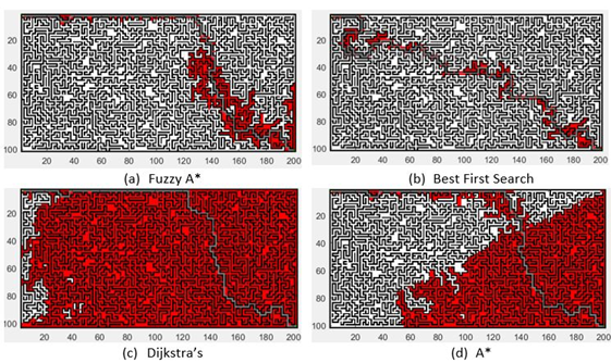
Figure 2. Path Planning Result for coordinates (0.0) to (200.100)
We employed randomly generated maps with specific constraints to mimic real-world path planning challenges. These constraints, including the positioning of start and end points and the distribution of obstacles, are designed to replicate common scenarios encountered in autonomous navigation. The chosen constraints are reflective of situations where path planning must account for unpredictable environments and limited maneuverability, thus providing a rigorous test for our algorithm. The randomly generated maps have 20301 vertices, 10548 non-obstacle vertices, and 9753 obstacle vertices, with 50 percent of the paths comprising obstacles and a dead-end environment. When establishing the strong direction parameter, other factors, such as the visited vertex's memory and the number of obstacles, will be considered in addition to the direct true direction. The experiment employs 100 maps with  (width x Height) dimensions, and the beginning and ending coordinates are fixed and determined at random. The constraints include several restrictions, such as (i) the position of start coordinate and goal coordinate must be on the last comer in opposite directions, (ii) the direct length between start and goal coordinates must be at least half the width or height of the map, and (iii) the area separated by the position of start coordinate and goal coordinates must contain at least 40 percent of the total number of obstacles shown in the Figure 3.
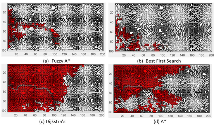
Figure 3. The Results of the Fuzzy A* method comparing with other methods for coordinates  and
and 
Table 1 contains the comparison findings for eight algorithms, including Dijkstra's, Breadth First Search (BFS), Depth First Search (DFS), Bidirectional BFS (BIBFS), Bidirectional DFS (BIDFS), Best First Search (BEFS), Bidirectional BEFS (BIBEFS), A*, and the Fuzzy A* method. Each approach yields the average path length and number of visited vertices based on 100 total path length and visited vertex studies. In addition, we display the degree of path suboptimality based on Dijkstra and Breath First Search.
Table 1. Comparison result
Algorithm | Path Length | Visited Node | Execution Time | Path Suboptimality | 
|
Djikstra's | 208 | 7181 | 207.02 | Optimal | 1 |
BFS | 208 | 7185 | 239.22 | Optimal | 1.00055 |
DFs | 1393 | 5758 | 231.59 | 6.7 x Optimal | 0.8018 |
BEFS | 257 | 492 | 13.69 | 1.23 x Optimal | 0.0685 |
BIBFS | 208 | 4600 | 515.118 | Optimal | 0.640 |
BHFS | 878 | 2261 | 3198.83 | 4.22 x Optimal | 0.314 |
BIBES | 257 | 749 | 38.36 | 1.23 x Optimal | 0.104 |
A* | 217 | 6438 | 202.82 | 1.043 x Optimal | 0.896 |
A* with admissible heuristic | 208 | 
| 131.07 | Optimal | 0.53 |
Fuzzy A* | 209 | 
| 86.04 | 1.0048 x Optimal | 0.375 |
Our analysis delves into the specific features of the Fuzzy A* method that contribute to its superior performance. We focus on how the Strength Direction parameter and Fuzzy Inference method dynamically optimize pathfinding, leading to reduced execution time and shorter path lengths without compromising optimality. Fuzzy algorithm is faster than all other algorithms, except for Best First Search (BEFS) and Bidirectional Best First Search, as seen in Table 1. (BIBEFS). However, this method resulting 1.23  optimal, indicating that the average created route is 1.23 times longer than the optimal path (208 vertices). In contrast, the Fuzzy A* method may yield
  Optimal path (209 vertices), which is a lesser number than BEFS and BIBEFS.
Fuzzy uses  , and
, and  more efficient vertices and less execution time than Dijlstra's, , and with an appropriate heuristic, respectively, while ensuring a high degree of suboptimality. Evidently, the proposed algorithm can dynamically alter the cost and efficiently estimate the value of the heuristic function. In addition, the proposed method does not necessitate laborious data collection, preprocessing, validation, trial-and-error modification of complex hyper parameters, or training. Instead, the cost is modified
using the Fuzzy Inference method and the Strength Direction parameter.
- CONCLUSION
In addressing real-world challenges such as obstacle avoidance, memory consumption, and time-sensitive operations, our study highlights the potential of the Fuzzy A* method in path planning. While traditional A* with admissible heuristics demonstrates commendable performance, our approach, through the introduction of the Strength Direction parameter, effectively balances computational time, memory efficiency, and near-ideal pathfinding. This is achieved by dynamically adjusting the searching cost and heuristic values through weakPowerDirection and strongPowerDirection parameters. However, it's important to acknowledge that the current parameter settings are based on expert knowledge and observations, which may limit the method's adaptability in environments with varying characteristics. To enhance the robustness and flexibility of our approach, future work will delve into optimizing the Strength Direction parameter using more sophisticated methods, potentially integrating adaptive learning techniques. This will allow the Fuzzy A* method to better adjust to diverse and unpredictable scenarios, further enhancing its applicability across various domains. From a practical standpoint, while the Fuzzy A* method shows promise, it's crucial to consider the implementation complexities in different real-world applications. Future research will also explore these practical aspects, focusing on simplifying the integration process and ensuring that the method can be efficiently applied in diverse operational environments without extensive customization. Moreover, we plan to rigorously test the robustness of the Fuzzy A* method under a range of conditions, including highly dynamic and unpredictable environments. This will provide deeper insights into its effectiveness and limitations, guiding further refinements. In conclusion, our research contributes a novel approach to path planning, balancing efficiency and performance. The Fuzzy A* method, with its innovative use of the Strength Direction parameter, offers a promising solution to complex pathfinding challenges. However, continuous improvement and adaptation are necessary to fully realize its potential in varying real-world applications. As we move forward, our focus will remain on optimizing, validating, and ensuring the practical applicability of this method, thereby contributing to the broader field of autonomous navigation and robotics.
REFERENCES
- B. K. Oleiwi, A. Mahfuz and H. Roth, "Application of Fuzzy Logic for Collision Avoidance of Mobile Robots in Dynamic-Indoor Environments," 2021 2nd International Conference on Robotics, Electrical and Signal Processing Techniques (ICREST), pp. 131-136, 2021, https://doi.org/10.1109/ICREST51555.2021.9331072.
- C. S. Tan, R. Mohd-Mokhtar and M. R. Arshad, "A Comprehensive Review of Coverage Path Planning in Robotics Using Classical and Heuristic Algorithms," in IEEE Access, vol. 9, pp. 119310-119342, 2021, https://doi.org/10.1109/ACCESS.2021.3108177.
- K. He, L. He, L. Fan, X. Lei, Y. Deng and G. K. Karagiannidis, "Efficient Memory-Bounded Optimal Detection for GSM-MIMO Systems," in IEEE Transactions on Communications, vol. 70, no. 7, pp. 4359-4372, 2022, https://doi.org/10.1109/TCOMM.2022.3176649.
- A. A. Z. Ibrahim, F. Hashim, A. Sali, N. K. Noordin and S. M. E. Fadul, "A Multi-Objective Routing Mechanism for Energy Management Optimization in SDN Multi-Control Architecture," in IEEE Access, vol. 10, pp. 20312-20327, 2022, https://doi.org/10.1109/ACCESS.2022.3149795.
- K. L. Keung, L. Xia, C. K. M. Lee and C. Y. Leung, "A Shortest Path Graph Attention Network and Non-traditional Multi-deep Layouts in Robotic Mobile Fulfillment System," 2022 IEEE International Conference on Industrial Engineering and Engineering Management (IEEM), pp. 0655-0659, 2022, https://doi.org/10.1109/IEEM55944.2022.9989607.
- L. Zhe, L. Yibin, R. Xuewen, and Z. Hui, “Path Planning Based on ADFA∗ Algorithm for Quadruped Robot,” IEEE Access, vol. 7, pp. 111 095–111 101, 2019, https://doi.org/10.1109/ACCESS.2019.2920420.
- J. Yang, J. Ni, M. Xi, J. Wen and Y. Li, "Intelligent Path Planning of Underwater Robot Based on Reinforcement Learning," in IEEE Transactions on Automation Science and Engineering, vol. 20, no. 3, pp. 1983-1996, 2023, https://doi.org/10.1109/TASE.2022.3190901.
- J. Yang, J. Huo, M. Xi, J. He, Z. Li and H. H. Song, "A Time-Saving Path Planning Scheme for Autonomous Underwater Vehicles With Complex Underwater Conditions," in IEEE Internet of Things Journal, vol. 10, no. 2, pp. 1001-1013, 2023, https://doi.org/10.1109/JIOT.2022.3205685.
- T. T. Cam Giang, N. T. Dung, H. T. Thanh Binh, D. Q. Huy and M. T. Thoa, "Wave Environment Decomposition with Adaptive Tri-Objective Particle Swarm Optimization for Mobile Robot Path Planning," 2022 IEEE Symposium Series on Computational Intelligence (SSCI), pp. 990-997, 2022, https://doi.org/10.1109/SSCI51031.2022.10022243.
- J. Liu, C. -W. Pui, F. Wang and E. F. Y. Young, "CUGR: Detailed-Routability-Driven 3D Global Routing with Probabilistic Resource Model," 2020 57th ACM/IEEE Design Automation Conference (DAC), pp. 1-6, 2020, https://doi.org/10.1109/DAC18072.2020.9218646.
- T. A. Ayall et al., "Graph Computing Systems and Partitioning Techniques: A Survey," in IEEE Access, vol. 10, pp. 118523-118550, 2022, https://doi.org/10.1109/ACCESS.2022.3219422.
- Z. Yao, W. Wang, J. Zhang, Y. Wang and J. Li, "Jump Over Block (JOB): An Efficient Line-of-Sight Checker for Grid/Voxel Maps With Sparse Obstacles," in IEEE Robotics and Automation Letters, vol. 8, no. 11, pp. 7575-7582, 2023, https://doi.org/10.1109/LRA.2023.3320435.
- E. P. Herrera-Alarcón, M. Satler, M. Vannucci and C. A. Avizzano, "GNGraph: Self-Organizing Maps for Autonomous Aerial Vehicle Planning," in IEEE Robotics and Automation Letters, vol. 7, no. 4, pp. 10721-10728, 2022, https://doi.org/10.1109/LRA.2022.3195192.
- S. Franco, J. Sustarevas and S. Bernardini, "Hybrid Discrete-Continuous Path Planning for Lattice Traversal," 2022 IEEE/RSJ International Conference on Intelligent Robots and Systems (IROS), pp. 8971-8978, 2022, https://doi.org/10.1109/IROS47612.2022.9981801.
- Z. Husain, A. Al Zaabi, H. Hildmann, F. Saffre, D. Ruta, and A. F. Isakovic, "Search and Rescue in a Maze-like Environment with Ant and Dijkstra Algorithms," in Drones, vol. 6, no. 10, Art. no. 273, 2022, https://doi.org/10.3390/drones6100273.
- S. Zhang, Y. Li, F. Ye, X. Geng, Z. Zhou, and T. Shi, "A Hybrid Human-in-the-Loop Deep Reinforcement Learning Method for UAV Motion Planning for Long Trajectories with Unpredictable Obstacles," in Drones, vol. 7, no. 5, Art. no. 311, 2023, https://doi.org/10.3390/drones7050311.
- W. He, Z. Cao, and H. Ye, "Path Planning Algorithms for Mobile Robots in Hospital Environment during Covid-19," in Proceedings of the 3rd International Symposium on Artificial Intelligence for Medicine Sciences (ISAIMS '22), pp. 522-530, 2022, https://doi.org/10.1145/3570773.3570853.
- S. Kim and B. An, "Learning Heuristic A: Efficient Graph Search using Neural Network," 2020 IEEE International Conference on Robotics and Automation (ICRA), pp. 9542-9547, 2020, https://doi.org/10.1109/ICRA40945.2020.9197015.
- M. P. Strub and J. D. Gammell, "Adaptively Informed Trees (AIT*) and Effort Informed Trees (EIT*): Asymmetric bidirectional sampling-based path planning," in Int. J. Rob. Res., vol. 41, no. 4, pp. 390-417, 2022, https://doi.org/10.1177/02783649211069572.
- J. Li and X. Wu, "Constrained Shortest Path by Parameter Searching," 2019 2nd International Conference on Safety Produce Informatization (IICSPI), pp. 26-29, 2019, https://doi.org/10.1109/IICSPI48186.2019.9095897.
- J. Persis, “A novel routing protocol for underwater wireless sensor network using pareto uninformed and heuristic search techniques,” Wireless Personal Communications, vol. 121, no. 3, pp. 1917-1944, 2021, https://doi.org/10.1007/s11277-021-08747-y.
- M. Chen and D. Zhu, "Optimal Time-Consuming Path Planning for Autonomous Underwater Vehicles Based on a Dynamic Neural Network Model in Ocean Current Environments," in IEEE Transactions on Vehicular Technology, vol. 69, no. 12, pp. 14401-14412, 2020, https://doi.org/10.1109/TVT.2020.3034628.
- P. Lehner and A. A.-S. affer, “The Repetition Roadmap for Repetitive Constrained Motion Planning,” IEEE Robotics and Automation Letters, vol. 3, no. 4, pp. 3884–3891, 2018, https://doi.org/10.1109/LRA.2018.2856925.
- R. Kong and X. Tong, "Anytime Dynamic Heuristic Search for Suboptimal Solution on Path Search," 2020 13th International Congress on Image and Signal Processing, BioMedical Engineering and Informatics (CISP-BMEI), Chengdu, China, 2020, pp. 1070-1074, https://doi.org/10.1109/CISP-BMEI51763.2020.9263589.
- J. Wang, N. Wu, W. X. Zhao, F. Peng, and X. Lin , “Empowering A∗ Search Algorithms with Neural Networks for Personalized Route Recommendation,” in Proceedings of the 25th ACM SIGKDD international conference on knowledge discovery & data mining, pp. 539-547, 2019, https://doi.org/10.1145/3292500.3330824.
- Y. Wang, S. Wang, Y. Xie, Y. Hu and H. Li, "Q-learning-based Collision-free Path Planning for Mobile Robot in Unknown Environment," 2022 IEEE 17th Conference on Industrial Electronics and Applications (ICIEA), pp. 1104-1109, 2022, https://doi.org/10.1109/ICIEA54703.2022.10006304.
- X. Wang, Z. Ning, S. Guo and L. Wang, "Imitation Learning Enabled Task Scheduling for Online Vehicular Edge Computing," in IEEE Transactions on Mobile Computing, vol. 21, no. 2, pp. 598-611, 1 Feb. 2022, https://doi.org/10.1109/TMC.2020.3012509.
- S. Choudhury, D. Dey, M. Bhardwaj, S. Arora, A. Kapoor, G. Ranade, and S. Scherer, “Data-driven planning via imitation learning,” The International Journal of Robotics Research, vol. 37, no. 13-14, pp. 1632–1672, 2018, https://doi.org/10.1177/0278364918781001.
- P. Cai, S. Wang, Y. Sun and M. Liu, "Probabilistic End-to-End Vehicle Navigation in Complex Dynamic Environments With Multimodal Sensor Fusion," in IEEE Robotics and Automation Letters, vol. 5, no. 3, pp. 4218-4224, 2020, https://doi.org/10.1109/LRA.2020.2994027.
- M. Mia et al., “Identifying factors affecting irrigation metrics in the Haor basin using integrated Shannon's entropy, fuzzy logic and automatic linear model,” Environmental Research, vol. 226, p. 115688, 2023, https://doi.org/10.1016/j.envres.2023.115688.
AUTHOR BIOGRAPHY

| Gregorius Airlangga received the B.S. degree in information system from the Yos Sudarso Higher School of Computer Science, Purwokerto, Indonesia, in 2014, and the M.Eng. degree in informatics from Atma Jaya Yogyakarta University, Yogyakarta, Indonesia, in 2016. He got Ph.D. degree with the Department of Electrical Engineering, National Chung Cheng University, Taiwan. He is also an Assistant Professor with the Department of Information System, Atma Jaya Catholic University of Indonesia, Jakarta, Indonesia. His research interests include artificial intelligence and softwareengineering include path planning, machine learning, natural language processing, deep learning, software requirements, software design pattern and software architecture.
|
Fuzzy A* for optimum Path Planning in a Large Maze (Gregorius Airlangga)