ISSN: 2685-9572 Buletin Ilmiah Sarjana Teknik Elektro
Vol. 8, No. 5, October 2026, pp. 1700-1723
Telling Faults from Attacks: A Gain-Matched Dual-Residual Observer with Guaranteed Detection Bounds for Unmanned Aerial Vehicles
Mohammed Jasim Mohammed
Department of Medical Instrumentation Techniques Engineering, Technical Engineering College, Al-Kitab University, Altun Kupri, Kirkuk, 36001, Iraq
ARTICLE INFORMATION |
| ABSTRACT |
Article History: Received 17 July 2026 Revised 26 October 2026 Accepted 10 November 2026 |
| 
The reason for loss of thrust is either degradation of the unmanned aerial vehicle's hardware or an interfering adversary, requiring opposite responses yet the single-residual diagnoser cannot distinguish between the two reasons. Research contribution is a dual-residual observer which is designed to detect anomalies in the actuation path as well as sensing path, a physical-admissibility test that differentiates faults from attacks, and detection bounds that are satisfied under specified bounds of disturbances and noise. Two Luenberger observers with the same gains are driven by commanded and measured rotor thrust; the difference between the two is proven to be invariant to all sensor-path signals and it is demonstrated that gain matching is required. If an adversary were to manage to suppress this residual, they would also have to excite the second one. The passive degradation is modeled as dissipative and independent of time and therefore an exact description of a non-empty set of attacks indistinguishable from faults. The validation was conducted using 450 Monte Carlo simulation runs of a linearised quadrotor model about the hover state with 25 model parameters tuned by 6 metaheuristic optimisers. There was no false alarm under the whale optimization algorithm tuned design and disturbances were within the assumed bounds; a false alarm error rate of 0.125 was observed when disturbance was increased by 1.5 times the assumed bounds. It successfully identified 82.9% of anomalous runs (96.7% without the linear GNSS drift) with a mean delay of 63 ms, and distinguished faults from attacks using 0.854 balanced accuracy and Matthews correlation of 0.696. In all runs, 11 anomaly families were detected and eight were also classified correctly, with no detections of slow GNSS drift and spoofing. Detection sensitivity is not the key difference between a fault and an attack; HIL validation is still a requirement. |
Keywords: Unmanned Aerial Vehicle; Fault-Attack Discrimination; Residual Generation; Cyber-Physical Security; Guaranteed Detection Bounds |
Corresponding Author: Mohammed Jasim Mohammed, Department of Medical Instrumentation Techniques Engineering, Technical Engineering College, Al-Kitab University, Altun Kupri, Kirkuk, 36001, Iraq. Email: dr.mohammed.jasim@uoalkitab.edu.iq |
This work is open access under a Creative Commons Attribution-Share Alike 4.0 
|
Document Citation: M. J. Mohammed, “Telling Faults from Attacks: A Gain-Matched Dual-Residual Observer with Guaranteed Detection Bounds for Unmanned Aerial Vehicles,” Buletin Ilmiah Sarjana Teknik Elektro, vol. 8, no. 5, pp. 1700-1723, 2026, DOI: 10.12928/biste.v8i5.17456. |
INTRODUCTION
Motivation
Today, small unmanned aerial vehicles (UAVs) have been introduced to the field of infrastructure inspection, precision agriculture, logistics and wildfire response and surveillance, to such an extent that their reliability is no longer an engineering topic, but a public-safety one [1]-[4]. This same expansion has increased the target area for hackers. A modern airframe reveals a number of command-and-control links, satellite-navigation receiver, identification broadcast and payload data path, all of which have been shown to be field exploitable [1],[5][6]. There are two themes to some of the reviews of UAV cyber security: navigation-related risks are the primary residual risk and most published countermeasures are only validated in simulation and are too demanding for the class of vehicle for which they are designed [1],[7].
The operational problem tackled in this paper is more specific and focused than the problem "detect anomalies". What about a vehicle that has 30 % loss of thrust on rotor 2 reported by the diagnostics? If the problem is a chipped blade, the proper answer is to re-distribute the thrust over the remaining rotors, and to continue with the mission; termination of that mission is an unnecessary loss of availability and, in a populated area, a hazard. If it is an injection on the command link, reallocation is the exact wrong move since the reallocation law is based on commands which the opponent can control, and an attacker who can inject the first channel can inject the others. The same measure thus gives two answers, which are not only different, but contradictory answers. If it's installed to deal with them in those situations, a diagnostic layer that can't tell them apart is not incomplete, it's just a hindrance.
Two phrases are repeated in the story. An observer is a copy of the model of the vehicle that is run concurrently with the autopilot, and the prediction it makes of the measurement that should be detected by the sensors would be small if everything was fine, but would get bigger if it didn't. Model based diagnosis alerts to alarms if a residual exceeds a threshold.
This paper distinguishes three tasks, which are usually combined in one. Anomaly detection is used to determine if something is amiss and is quantified by the true positive rate (TPR), false alarm rate (FAR) and detection delay. The channel's accuracy dictates the channel's usefulness for the anomaly and whether it enters through the actuation path (commands, rotors and telemetry) or the sensing path (navigation and attitude sensors). Fault-versus-attack classification decides whether the anomaly is physical degradation or adversarial interference and is measured by balanced accuracy and the Matthews correlation coefficient (MCC), both insensitive to class imbalance. The adversary is assumed able to read, modify and replay traffic on the command, sensor and actuator-telemetry links, but not to alter the physics of the airframe; Section 2.2 states this boundary precisely [6],[8].
Related Work
Observer-based fault diagnosis. Fault diagnosis for multirotors is mature [4]. Disturbance observers, extended state observers and sliding-mode observers reconstruct actuator effectiveness and sensor bias with high fidelity, and the resulting estimates drive fault-tolerant controllers that keep a damaged vehicle flying [9]–[11]. Hu et al. combine an integral sliding surface with a disturbance observer so that actuator faults and wind are compensated simultaneously [9]. Nguyen and Pitakwachara use an adaptive sliding-mode observer to estimate actuator and sensor faults and feed an integral terminal sliding-mode reconfiguration law [10], and estimate sensor faults for attitude fault-tolerant control [12]. Mai et al. extend the idea to compound faults through a nonlinear extended state observer with prescribed performance guarantees [11]. Some works are related to the application of high-order sliding-mode disturbance observers to the attitude control system under actuator dynamics [13], the extension of state observers to the formation flight problem in the wake vortex environment [14] and experimental validation of the disturbance-observer-based sliding-mode controller under the conditions of turbulent indoor environment [15]. A second line of work evaluates residuals with sets rather than fixed thresholds: interval observers isolate quadrotor actuator faults with experimentally validated bounds [16], zonotopic set-membership estimators detect faults in underwater and space vehicles [17][18], and set-invariance analysis yields the minimum detectable and isolable faults of linear-parameter-varying (LPV) vehicle models [19]. Data-driven linear models obtained with the Koopman operator have also been paired with Luenberger observers to isolate multirotor actuator faults beyond a single linearisation [20].
Data-driven fault diagnosis. In parallel, learning-based diagnosis has become competitive. Cascaded deep networks localise failed actuators on highly redundant multirotors to within one rotor [21], evidence-theoretic fusion classifies unmanned-system fault types under conflicting sensor evidence [22], and off-board vibration analysis diagnoses rotor faults without consuming onboard computation [23], while onboard vibration and inertial data detect small propeller faults in real time [24][25].
Most schemes in both groups assume, implicitly, that the anomaly they reconstruct is benign in origin. The reconstructed signal is passed directly to reallocation, and no test is applied to ask whether hardware degradation could have produced it.
Security-oriented detection. Attack detection for UAVs has grown from the opposite direction and is largely data-driven. Stacked ensembles, adversarial-training models, recursive feature elimination and multi-channel receiver analysis achieve high accuracy on spoofing datasets [26]–[29]; broader surveys catalogue the jamming and spoofing landscape [30] and the role of learning in satellite navigation [31]; deep models detect spoofed satellite signals on small UAVs [32]; and graph neural networks with attention detect anomalies in unmanned-system telemetry [33]. Learned detectors are themselves exposed to adversarial manipulation [34], and their false-alarm rates are properties of the evaluation data rather than guarantees [35]. Model-based alternatives exist: observers detect and compensate attacks on a UAV’s desired trajectory [36], neural observers protect UAV formations against deception attacks [37], and robust H∞ observers estimate actuator and sensor attacks jointly with the state of a stochastic quadrotor [38]. Beyond the UAV literature, the cyber-physical systems community has built a substantial theory of denial-of-service, false-data-injection and replay attacks [8],[39], covering secure state estimation [40]–[42], safety-constrained control under injection [43], observer-based estimation of injected signals [44], localisation of latent injections in distributed cluster control [45], distributed detection across large sensor networks [46], secure state estimation and recovery under deliberately stealthy attacks [47], and learning-based reconstruction of tampered measurements [48]. Resilient controllers that tolerate cyberattacks and actuator faults simultaneously have recently been designed for fixed-wing UAV formations [49].
These methods answer “is something wrong?” with considerable skill, and several tolerate attacks and faults together. Most do not answer “is this a broken rotor or an intruder?”, because a classifier trained on labelled attack traffic, or a controller that compensates every disturbance alike, has no physical model against which to test whether an observation is producible by hardware degradation.
Research Gap
A small body of work addresses discrimination directly. Hu et al. use a pair of distributed disturbance-decoupling observers to detect and identify both device faults and data-injection attacks in multi-agent systems [50]. Zhang et al. separate sensor replay attacks from sensor bias faults with a specially designed watermark and adaptive estimation [51], and Badr et al. discriminate faults from replay attacks in hybrid systems by stochastic coding combined with adaptive and sliding-mode observers [52]. These methods show that discrimination is possible, but each relies on an added signal (a watermark or a code) or on network structure, treats one attack class, and sets its thresholds statistically or empirically. None does not think of an opponent that steals actuator telemetry, and none says the set of attacks that it can't isolate from faults.
The gap discussed here is therefore one of geometry of the remaining space, not some learned decision boundary, or an injected watermark; and, in this case, the guarantees are shown assuming particular conditions, not measured. A comparison of the present work with representative methods is provided in Table 1 and a comparison of reported results is provided in Section 3.7. The method is further developed in Section 2, and a simulation study is reported and discussed in Section 3, before conclusions are drawn in Section 4.
Research Contribution
The research contribution was a diagnostic observer with the difference between a hardware error and a cyber-attack being a structural property not a learned one. It consists of three parts, that include a theorem, and a measured consequence.
C1 — Dual Residuals that are exactly decoupled and Coverage of forged Telemetry. The difference residual for two Luenberger observers with commanded and measured rotor thrust is exactly invariant to all of the sensor-path signals and is only dependent on the discrepancy in the sensor actuation (Theorem 1). It is proved that gain matching is forced (Theorem 2) and that if the adversary succeeds in deactivating this residual, then he must activate the second one (Theorem 3). With mismatched gains, the sensor leakage in simulation is 4 × 10⁷ times the threshold, and forged telemetry is always detected.
C2 — Physical admissibility discrimination: Blind statement. Any noticeable change or actuator that adds thrust or whose parameters change over the observation period is considered an attack, as passive actuator degradation is dissipative and time invariant. The attacks that can't be separated from faults are characterised exactly (Theorem 5), and precision of the estimation is correlated with the command excitation (Theorem 6). The balanced accuracy reduces to 0.670 when the dual structure is removed.
C3 — Deterministic detection — guaranteed with given bounds. When wind, measurement noise and telemetry noise are within assumed bounds, together with closed-form minimum detectable anomalies (Theorem 4), peak-gain thresholds give zero false alarms. In simulation the bounds are conservative by factors of 1.7–3.2, and false alarms appear when the true disturbance exceeds the assumed bound by 50 %.
Luenberger observers, residual thresholds and metaheuristic tuning are established tools; the contribution lies in their gain-matched pairing and the guarantees it admits. Six population-based optimisers are compared only as a means of designing the 25 free parameters. The method is not a universal discriminator: Theorem 5 identifies a non-empty class of dissipative, affine, time-invariant attacks that remain indistinguishable from actuator faults, and slow sensor drift lies below the detection bound of Theorem 4. All results are obtained by simulation of a hover-linearised quadrotor model.
Table 1. Properties of representative methods compared with the present work
Method Family | Fault/Attack Discrimination | Channels Covered | Model or Data | Detection Threshold | Blind Spots Characterised |
Disturbance, extended-state and sliding-mode observer FTC [9]–[13] | No; anomaly compensated whatever its origin | Actuator; sensor in [12] | Nonlinear model | Empirical | Not stated |
Interval and zonotopic set-based observers [16]–[19] | No (faults only) | Actuator or parametric faults | Linear or LPV model, bounded uncertainty | Set-based, guaranteed under bounds | Minimum detectable faults [19] |
Learning-based fault diagnosis [21][22],[24] | No (faults only) | Actuator, rotor, propeller | Labelled data | Learned | Not stated |
Learning-based spoofing detection [26][27],[32] | No (attacks only) | GNSS | Labelled data | Learned; empirical false-alarm rate | Not stated |
Observer-based attack detection and resilient control [36],[38],[49] | No; attacks (and faults in [49]) compensated jointly | Command, actuator, sensor | Model | Empirical or H∞-based | Not stated |
Fault/attack discrimination [50]–[52] | Yes, for injection or replay attacks | Network, sensor | Model plus decoupling, watermark or coding | Statistical or empirical | Not stated |
This work | Yes, by physical admissibility | Actuation and sensing, separated exactly | Hover-linearised model, bounded noise | Deterministic peak-gain; zero false alarms under bounds | Exact indistinguishable set; drift bound |
METHOD
Figure 1 summarises the research methodology. The outer loop is the offline design of the diagnostic layer by metaheuristic optimisation (Algorithm 2); nested within it is the runtime pipeline that executes onboard at every sample,  s (100 Hz), as Algorithm 1. After an alarm,
 = 130 samples (1.3 s) are collected before the fault-versus-attack verdict is issued. The remainder of this section develops each block in turn; each block of Figure 1 carries the number of the equation that defines it.
Vehicle model
A quadrotor in  configuration is linearised about hover. The state is
| 
| (1) |
comprising north-east-down position, body velocity, Euler attitude and body rates. The input is the vector of four rotor thrusts  taken about the hover trim
 , so that a loss of effectiveness acts multiplicatively on individual entries — a choice that matters, because the multiplicative structure is exactly what the discrimination test in Section 2.6 exploits. Rotor thrusts map to the wrench through the mixer
| 
| (2) |
with arm length  and yaw-torque coefficient
 . The continuous dynamics are
 with
 , where
 distributes collective thrust onto
 and the three torques onto the angular accelerations, and
 injects a wind force onto the translational axes. Zero-order-hold discretisation at
 yields
 . The measured output is
| 
| (3) |
with  selecting
 , so
 from a satellite receiver, an attitude reference and a rate gyro. (3) makes explicit that sensor faults and sensor injection enter additively at the output and are indistinguishable at this level. Table 2 lists all parameters.
The mass, inertia and arm length in Table 2 describe a 1.2 kg quadrotor with 0.46 m between diagonal rotors; at hover each rotor carries mg/4 = 2.94 N, well inside the 7.5 N limit. The wind, measurement-noise and telemetry-noise bounds are the quantities on which the zero-false-alarm guarantee of Theorem 4 rests (Assumption AS2 in Table 3). The rotor-telemetry bound ν̄ = 0.020 N is 0.7 % of hover thrust; as explained in Section 2.2, the bound can be loosened to decrease the limits of detection, and also the rotor-telemetry bound can be modified to yield a more favorable value.
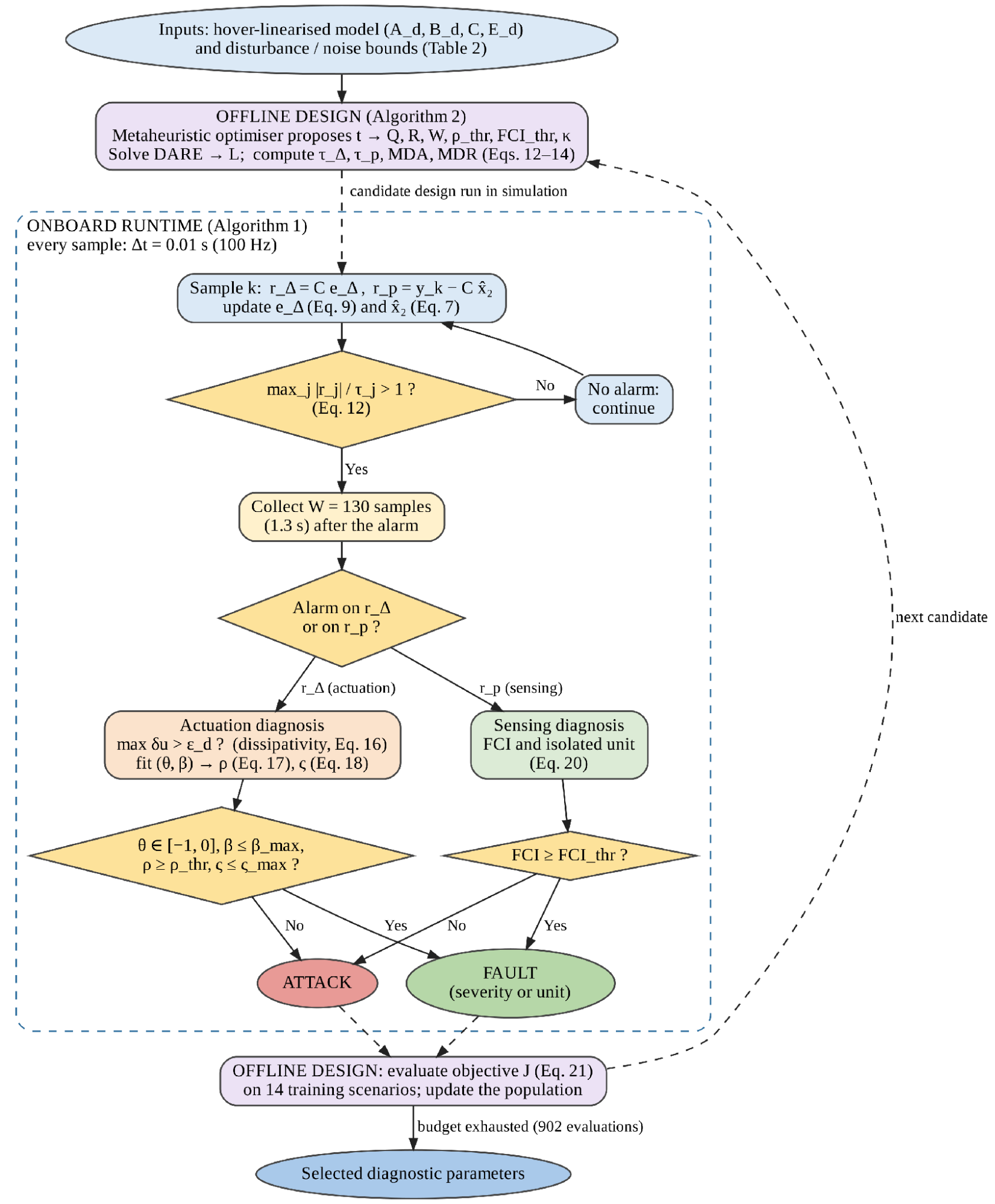
Figure 1. Research methodology: offline design of the diagnostic layer (Algorithm 2) and the onboard runtime pipeline executed every = 0.01 s (Algorithm 1). Equation numbers identify the defining relation of each block
Table 2. Vehicle, sensor and disturbance parameters
Parameter | Value | Unit |
Mass  | 1.20 | kg |
Gravity  | 9.81 | m/ |
Inertia  | 0.0123 | kg· |
Inertia  | 0.0224 | kg· |
Arm length | 0.23 | m |
Yaw-torque coefficient | 0.016 | m |
Translational drag  | 0.15 | 
|
Rotational drag  | 0.05 |
|
Per-rotor thrust limit | 7.5 | N |
Sampling interval | 0.01 | S |
Rotor-telemetry bound  | 0.020 | N |
Wind-force bound  | 1.20 | N |
GNSS noise bound | 0.06 / 0.06 / 0.09 | m |
Attitude noise bound | 2.0 / 2.0 / 3.0 ×  | rad |
Rate noise bound | 4.0 × | rad/s |
Fault and Threat Model
Let  ,
 , denote rotor effectiveness,
 an additive passive thrust offset,
 an injection on the controller-to-actuator link, and
 an injection on the sensor-to-controller link. Writing
 for the command computed by the autopilot, the thrust actually delivered is
| 
| (4) |
and the actuator-side telemetry, from electronic-speed-controller feedback, is
| 
| (5) |
unless the adversary also compromises the telemetry path, in which case  is whatever the adversary reports. (4) covers loss of effectiveness (
 ), total rotor loss (
 ), passive offset (
 ) and command injection (
 ) within a single expression. That unification is deliberate: it is what makes the admissibility argument of Section 2.6 possible, because fault and attack become distinguishable parameter regions of one model rather than separate models requiring separate detectors.
We assume a Dolev–Yao adversary on the communication links, able to read, modify and replay traffic on the command and sensor channels, and optionally on the telemetry channel, but unable to alter the physics of the airframe.
Security boundary. The adversary may read, modify and replay traffic on the command, sensor and telemetry links [6],[8]. It cannot change the airframe: propeller sabotage, physical tampering and electronic-speed-controller (ESC) firmware that alters the delivered thrust lie outside the model. Satellite-navigation signal spoofing is represented by its effect, an additive injection on the position measurement. Every guarantee below holds only inside this boundary.
Actuator-side telemetry. On current multirotors, is obtained from ESC telemetry: bidirectional digital ESC protocols report each motor’s electrical speed in real time, and open-source autopilots log it (see, e.g., the ArduPilot ESC-telemetry documentation, https://ardupilot.org/copter/docs/common-esc-telemetry.html). Thrust then follows as  with
 calibrated on a thrust stand, so
 must cover the calibration error of , speed quantisation and air-density variation. Because the actuation threshold
 in (12), and with it the minimum detectable actuation anomaly, scales linearly with , a bound of 2 % of hover thrust instead of 0.7 % would raise the 5.17 % loss-of-effectiveness bound of Table 9 to about 15 %. Speed-derived telemetry has one blind spot: a chipped or cracked propeller lowers at unchanged speed, so the thrust loss does not appear in δu and acts instead on the airframe, where it is seen by
 . A powertrain model [25] would return such a damage to the actuation channel if combined with the speed.
Fault-model scope. Passive degradation is shown as (4), and has parameters that remain constant over the classification window ( = 130 samples, 1.3 s). Both wear and thermal drift change on a minutes to hours time scale, while blade loss or motor failure is a step, so it is piecewise constant at this time scale [24]. The faults not included are not modelled: If a connector is loose, it is an intermittent fault, it is not time invariant; If an ESC fails at full throttle, it provides thrust and is not dissipative. Both would be considered attacks by the tests of Section 2.6 – the conservative one. The sensor models are defined as follows: bias (possibly due to a multipath jump on the GNSS receiver), drift (to receiver-clock drift instability or to an inertial bias instability), stuck output (due to a frozen data bus or driver), and injection (due to an adversary on the sensor link).
Table 3 summarizes assumptions underlying the theorems below and what occurs when each assumption is transgressed.
Table 3. Assumptions, the results that use them, and the consequence of violating them
ID | Assumption | Used by | If violated | Examined in |
AS1 | Hover-linearised model ( ,  , ,  ) shared by both observers | Theorems 1–4 | Theorems 1–3 still hold because both observers share the model; airframe mismatch enters and can cause sensing-channel false alarms | Section 3.6 |
AS2 | Bounded wind ( ), measurement noise (  ) and telemetry noise (  ) | Theorem 4 | False-alarm rate 0.125 at 1.5× and 1.000 at 2× the bound | Section 3.6, Figure 11 |
AS3 | Per-rotor thrust telemetry is available, honest or forged | Theorems 1–3 |  cannot be formed
| Section 2.2 |
AS4 | Delivered thrust follows the command without lag in nominal operation | Theorems 1 and 4(i) | Motor lag gives  in transients and can cause actuation false alarms unless modelled | Section 3.6 |
AS5 | Passive actuator faults are dissipative ( ) | Theorem 5, dissipativity test | Thrust-increasing faults (ESC runaway) are labelled attacks | Section 3.7.4 |
AS6 | Fault parameters are constant over = 130 samples (1.3 s) | Theorems 5–6, conformity test | Intermittent faults are labelled attacks | Section 3.7.4 |
AS7 | Sensor faults are confined to one unit and are bias plus drift | Eq. (20) | Multi-unit or other fault shapes are labelled attacks | Table 7 |
AS8 | No actuator saturation inside the conformity window | Theorem 6, Eq. (17) | Severity estimate degraded at low excitation | Figure 9 |
AS9 | The adversary cannot alter the physics of the airframe | Theorems 3 and 5 | Outside the scope of the method | — |
Gain-Matched Twin Observers
Define two observers sharing one gain  :
| 
| (6) |
| 
| (7) |
The first one is based on the autopilot's request, the second one is based on the airframe's input. The diagnostic signals are:
| 
| (8) |
Theorem 1 (Exact sensor decoupling). Let  . Then
| 
| (9) |
Thus, is a function of only  . It is free of y and hence of the state, the wind, the measurement noise, any sensor fault and any sensor injection.
Proof. Subtracting (6) from (7), the injection terms give  : the measurement
 cancels identically because the same multiplies it in both. The input terms leave
 . Finally
 . Since (9) contains no term in , and
 is initialised independently of , the trajectory of is determined by alone.

In physical terms, both observers receive the same measurement through the same gain, so whatever the sensors report — noise, a fault or a forged signal — cancels in their difference, and what remains is driven only by the mismatch between the thrust requested and the thrust reported. Because the cancellation uses only the model shared by the two observers, it holds even when that model differs from the real airframe (Assumption AS1); Section 3.6 discusses the one modelling error that does reach rΔ, actuator lag.
Theorem 2 (Necessity of gain matching). If the observers carry gains  , then
| 
| (10) |
and the leakage term  transports sensor-path signals into . Decoupling holds for arbitrary sensor signals if and only if
 .
Proof. Sufficiency is Theorem 1. For necessity, suppose 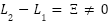 and pick a sensor injection such that
 , which is possible because
 has a unit direct feedthrough from by (11) below. Then depends on , contradicting decoupling.
Equation (10) identifies gain matching as a structural requirement rather than a tuning preference; Section 3.5 measures the consequence of violating it.
The complementary statement is deduced from the error dynamics of the second observer. With  ,
| 
| (11) |
Equation (11) contains no term in  , or
 : because observer 2 is propagated with the input the airframe actually received, actuation anomalies do not appear in except through the telemetry noise
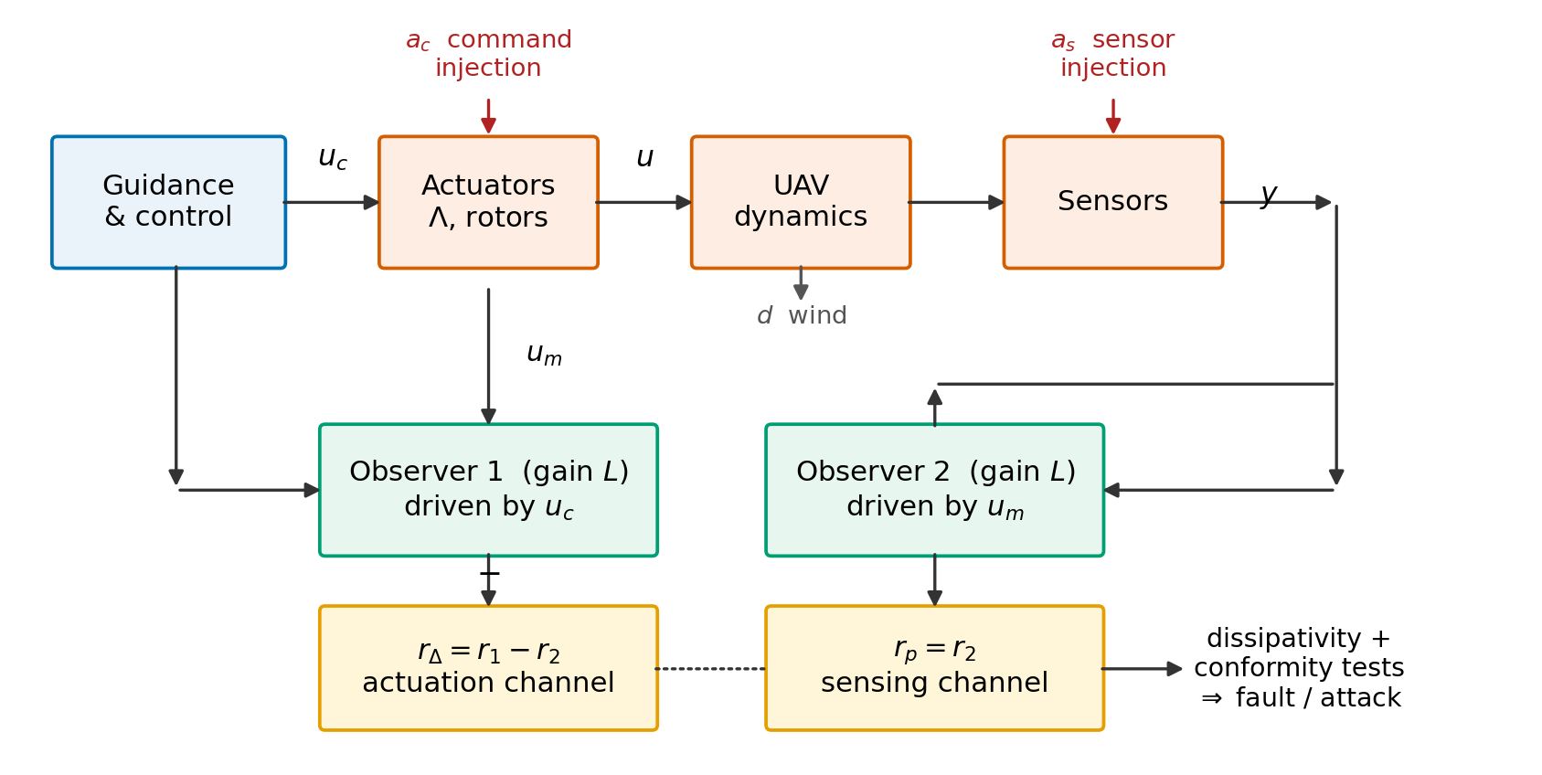
 . Figure 2 shows the resulting architecture. The two residuals partition the anomaly space — observes the actuation path exclusively, the sensing and airframe path exclusively.
Figure 2. Dual-residual diagnostic observer
Dual-Channel Coverage
Theorem 1 assumes honest telemetry. The interesting adversary does not provide it.
Theorem 3 (Coverage). Suppose the adversary controls both and the reported telemetry . Then  requires
 ; but substituting into the general form of (11) leaves
 driven by
 whenever the delivered thrust differs from the command, so the anomaly appears in . Consequently no actuation-path anomaly is simultaneously invisible in and unless
 , that is, unless no anomaly exists.
Proof. By (9),  under arbitrary excitation iff
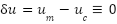 , i.e. . The term
 appearing in the error dynamics of observer 2 then becomes
 , which vanishes only if the delivered thrust equals the command. Hence invisibility in both residuals implies .
Theorem 3 is what elevates the architecture above the obvious alternative of thresholding  directly. That static test is simpler and, for honest telemetry, comparably sensitive; but it is defeated completely by a forging adversary, whereas the observer pair converts the forgery into a signal on the other channel. Section 3.5 confirms both halves of this statement experimentally.
Deterministic Thresholds and Detection Bounds
The nine residual channels carry different physical units, so thresholds are formed row-wise; a single scalar bound would set the attitude alarm at more than ten degrees and is unusable. Let  and let
 collect the row-wise
 norms of the corresponding impulse responses, that is, the induced
 gains. With
 a safety factor,
| 
| (12) |
where and  bound the wind force and the per-channel measurement noise. An alarm is declared when
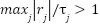 .
Theorem 4 (Zero false alarms and guaranteed detection). If  ,
 and
 , then in the anomaly-free case
 and
 for all
 , so the false-alarm rate is identically zero. Moreover:
- a persistent actuation discrepancy on rotor
 of magnitude is detected whenever
| 
| (13) |
- an abrupt sensor anomaly on channel
 is detected at the sample it occurs whenever
 , because the sensing channel has unit direct feedthrough,
 ;
- a sensor drift of rate
 on channel is detected whenever
| 
| (14) |
Proof sketch. The first claim is the definition of the induced  gain: each threshold in (12) is the worst-case peak of the corresponding residual channel over all admissible exogenous signals. For (i), the steady-state response to a constant
 is
 ; the anomaly is detected once its contribution to some channel exceeds the threshold by more than the worst-case noise contribution, giving the factor two. Claim (ii) follows from , so a step of magnitude appears undiminished in the residual at the sample of onset. For (iii), the asymptotic residual under a ramp of rate is
 , and the same margin argument applies.
Result (ii) is true and does not need to compute a gain. The awkward one is (14): a steady-state observer makes the DC gain of the sensor approach zero, and hence the  approach infinity. For this it is the only true shortcoming of the method, and is discussed in detail in Section 3.7.4.
Theorem 4 in practice means that you will only get silence on a healthy flight when wind and noise are within the limits of Table 2; Section 3.6 quantifies what happens beyond. The bounds are computed assuming the zero-order-hold model and are thus evaluated at the sampling points of the 100 Hz loop. The drift bound concerns a ramp, a near-DC signal which is well below the Nyquist frequency, 50 Hz, and the drift rate γ is the rate at which the injected error in the reported position grows, not the rate at which the airframe moves.
Discrimination on the Actuation Channel
Substituting (4) and (5) into  gives, per rotor,
| 
| (15) |
A passive degradation is characterised by two physical properties. It is dissipative — a failing rotor cannot produce more thrust than commanded, since rotor thrust scales as  and propeller damage, motor wear, ESC current limiting and battery sag all reduce
 or — and its parameters are properties of damaged hardware, hence constant over a short window. This motivates the admissible set
| 
| (16) |
Two tests follow. The dissipativity test declares an attack if 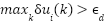 , since no member of (16) adds thrust; this test is unconditional and needs no window. The conformity test regresses
 on
 over samples, giving
 , a coefficient of determination
| 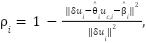
| (17) |
and a scale-invariant time-invariance index formed by fitting the two half-windows separately and comparing the discrepancy they predict,
| 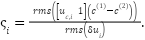
| (18) |
A fault is declared when  ,
 ,
 and
 ; otherwise an attack. Normalising by the anomaly magnitude in (18) is essential rather than cosmetic: an absolute bound on parameter drift is meaningless when commanded thrust swings by a factor of two under saturation, and using one causes total rotor loss to be misclassified despite a textbook fault signature. The estimate
 is returned as a severity estimate at no additional cost.
Theorem 5 (Exact indistinguishable set). In the noise-free case the actuation classifier declares “fault” if and only if  . An attack is classified as evasive if and only if it is dissipative and affine with constant coefficients (in which case it yields exactly the closed-loop trajectory of an admissible fault, and the FT-reallocation obtained for this fault is the proper response to this attack).
We state this plainly because it is the honest boundary of the method. An adversary can hide, but only by behaving indistinguishably from broken hardware, so its action space is reduced to dissipative, affine, time-invariant thrust reductions. This reduction is not harmless: on a quadrotor, a mimicked total rotor loss forces the same emergency as a real one. With noise, the envelope is widened by the test tolerances: a positive excursion below  , a parameter variation below
 and a non-affine component carrying less than 1 −
 = 3.1 % of the discrepancy energy also pass as faults. Mapping this envelope numerically over attack magnitude and time variation is left to future work.
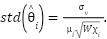
Theorem 6 (Identifiability). Let  and let the excitation index be
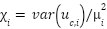 . The least-squares effectiveness estimate satisfies
| 
| (19) |
Proof. With the intercept included, the slope estimator has variance  . Substituting
 gives (19).
Equation (19) states that severity estimation and the rejection of slowly time-varying attacks both improve as the square root of command excitation, which is why a small zero-mean probing dither is superimposed on the rotor commands. Section 3.4 tests (19) directly. The dither is zero-mean, so it does not bias the commanded thrust, and by (19) its amplitude trades estimation precision against tracking error. It provides excitation rather than authentication, so an adversary who observes it gains nothing with respect to Theorem 6.
Discrimination on the Sensing Channel
A physical sensor fault must be able to be expressed as bias plus drift with a single sensor unit. Let  be the residual responses of (11) to a unit step and a unit ramp on channel . For each unit
 we solve a least-squares fit of the windowed residual, normalised channel-wise by
 , onto the dictionary
 , and record the best explained fraction
| 
| (20) |
If  , it is declared as a fault and the unit with the highest FCI value is returned as the isolated sensor, ie the isolation is free of charge when the classification is done. In just as much as (18): if it is not normalised, the position channels and attitude faults at the metre scale dominate the fit, and the attitude faults are systematically misread as attacks.
Algorithms
Per sample, Algorithm 1 needs about 708 multiply–accumulate operations for the present dimensions (12 states, 9 outputs, 4 rotors), that is, about 7.1 ×  per second at 100 Hz, plus one two-parameter least-squares fit over samples per alarm; its matrices occupy about 2.4 kB in single precision. This is a computational feasibility argument rather than a measured deployment; execution time on flight hardware has not yet been measured. Lines 4 and 6 are the key economy: requires no measurement at all.
Algorithm 1 DRDO runtime diagnosis |
1 given , , , , , , , ,  , ,  , 
2 ← 0;  ← 
3 for each sample k:
4 ←  ▹ actuation channel; no measurement used
5 ←  −  ▹ sensing channel
6 ← ( − ) + ( − ) ▹ Eq. (9)
7 ← + ( −  ) + ▹ Eq. (7)
8 if 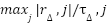 > 1 then channel ← ACTUATION; break
9 if  > 1 then channel ← SENSING; break
10 collect the samples following the alarm
11 if channel = ACTUATION:
12 ←   
13 if  : return ATTACK ▹ dissipativity, Eq. (16)
14 fit 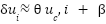 ;  by (17);  by (18)
15 if  and  and  :
return FAULT, severity 
16 else return ATTACK
17 else:
18 compute FCI and the maximising unit by (20)
19 if  ≥ : return FAULT, isolated unit
20 else return ATTACK |
Design Optimization
Twenty-five parameters remain free: twelve process weights and nine measurement weights defining through the filter Riccati equation, the window , the two conformity thresholds and  . Parameterising through the Riccati solution guarantees
 Schur for every admissible parameter vector, so the search is unconstrained in the stability sense — a practical advantage over optimising entrywise, where most of the search space is unstable. The objective aggregates sensitivity and decision quality,
| 
| (21) |
where  combines the normalised bounds of (13), Theorem 4(ii) and (14), and
 penalises class and channel errors on a fixed training set of fourteen scenarios. Six population-based optimisers are compared under an identical budget; settings are given in Table 4.
Table 4 lists the optimiser settings. Every algorithm receives the same budget of 902 objective evaluations — an initial population of 22 followed by 40 iterations of 22 — and is run ten times from independent random seeds; population-based optimisers of this kind are widely used to tune controller and estimator parameters [53]. The weights in (21) give the largest share to classification (0.45), because discrimination is the purpose of the method, then to sensitivity (0.30) and delay (0.20); the false-alarm term carries only 0.05 because Theorem 4 already fixes the false-alarm rate at zero under the design bounds. The tolerances ,  and are fixed rather than tuned.
Table 4. Optimiser settings. All six algorithms receive an identical evaluation budget
Setting | Value |
Population size | 22 |
Iterations | 40 |
Function evaluations per run | 902 |
Independent runs | 10 |
Search dimension | 25 |
PSO |  , 
|
DE | rand/1/bin,  ,  |
GA | SBX  , polynomial mutation  ,  ,  , elitist |
GWO | 
|
WOA | , spiral  |
CMA-ES |  ,  , 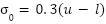
|
RESULT AND DISCUSSION
Experimental Setup
The closed loop uses a fixed linear-quadratic regulator and a fixed navigation observer, identical for every design, so that the optimiser tunes only the diagnostic layer and comparisons are not confounded by control performance. Fourteen anomaly families — seven physical-fault families and seven attack families Table 7 —and one anomaly-free nominal class are simulated with thirty Monte Carlo runs each — 450 runs — randomising magnitude, affected rotor or channel, onset time, wind and noise scaling, and seed. Because the loop samples at 100 Hz, oscillatory injections are represented only below the 50 Hz Nyquist frequency. A further family, the fault-mimicking attack of Theorem 5, is evaluated separately. Training and test sets are disjoint in seed, magnitude range and onset, so no result below is reported on data used for tuning. All results come from simulation of the hover-linearised model and do not demonstrate flight performance.
Optimizer Benchmark
Table 5 reports the statistics; Figure 3 shows the convergence behaviour and Figure 4 the dispersion of final objective values.
Every algorithm improves substantially on the untuned analytic design ( ). The more informative observation is that four of the six converge to within 0.07 % of one another at the optimum — 0.25332 for GWO, 0.25339 for PSO, 0.25340 for WOA and 0.25349 for DE. Agreement of that tightness across mechanistically dissimilar search strategies suggests that they reach a similar region of the search space, rather than that any one of them is superior; it does not establish global optimality. The Friedman test yields χ^2=11.543 and p=0.0416, which indicates the differences are significant at the 5 % level but they are for reliability and not for achievable quality.
The ranking for that axis is reversed. DE has the lowest mean (0.26050), standard deviation (0.01347) and Friedman rank. While having the tightest dispersion (0.01024), CMA-ES consistently converges towards a slightly suboptimal basin, but not towards the shared optimum (best 0.27253), and the Wilcoxon p=0.006 against DE is not a coincidence. GA has the lowest mean (0.29284) and the largest spread (0.03073) when compared to the leaders. PSO, GWO and WOA are statistically indistinguishable from DE (p=0.322, 0.193, 0.064).
These differences were put in perspective by using effect sizes. There is only small to moderate agreement between runs on the ranking (Kendall's coefficient of concordance is 0.23, or χ2/[N(k − 1)]). However, only CMA-ES (p = 0.030, r ≈ 0.87) and GA (p = 0.040, r ≈ 0.81) are still significantly worse, while WOA (p = 0.192), GWO and PSO (both 0.386) do not differ significantly from DE. Here r = Z/√N where Z is recovered from the two-sided p-value. The differences in the best objective value of the four top algorithms at best 0.07 % are not significant in practice.
These statistics are reflected in Figure 4. DE is the lowest, most compact box with two outlying runs; PSO has a similar spread with two poor runs, but hits the same floor as DE; GWO and WOA have a fairly broad range with medians around 0.272; GA has the widest range, with its median above the best runs of the others, and consistent with a convergence to a somewhat inferior region; and CMA-ES has a narrow box above the best runs of the others, consistent with a convergence to a slightly worse region.
This is because the practical reading is dependent on the design workflow and that's why we report more than a best-value column. If the design is only performed once, offline, with multiple restarts being affordable, GWO or PSO-based methods should be preferred due to their best-of-n behaviour. In cases where one run is to be trusted, such as an onboard or automatic reconfiguration after a change, DE is the place to go, as the worst run (0.29774) is still better than the median for GA. Lacking predictability, CMA-ES is an appealing option only when the remaining few percent of objective is the most important. All of this would have been masked by a single ‘winner' if we had just reported on best value alone, as is often the case in comparative analysis.
Table 5. Optimiser statistics over 10 independent runs. Friedman  ,
 (
 ,
 ); Wilcoxon signed-rank tests are two-sided against DE, the lowest-mean algorithm. Untuned analytic baseline

Algorithm | Best | Mean | Median | Worst | Std | Time/run (s) | Friedman rank | Wilcoxon  vs DE |
PSO | 0.25339 | 0.27117 | 0.26422 | 0.31708 | 0.02337 | 23.03 | 2.8 | 0.322 |
DE | 0.25349 | 0.26050 | 0.25611 | 0.29774 | 0.01347 | 22.93 | 2.2 | — |
GA | 0.25662 | 0.29284 | 0.28225 | 0.33587 | 0.03073 | 23.38 | 4.4 | 0.010 |
GWO | 0.25332 | 0.27506 | 0.27238 | 0.29820 | 0.02097 | 23.68 | 3.4 | 0.193 |
WOA | 0.25340 | 0.27879 | 0.27242 | 0.31625 | 0.02149 | 22.75 | 3.7 | 0.064 |
CMA-ES | 0.27253 | 0.28561 | 0.28156 | 0.30270 | 0.01024 | 23.86 | 4.5 | 0.006 |
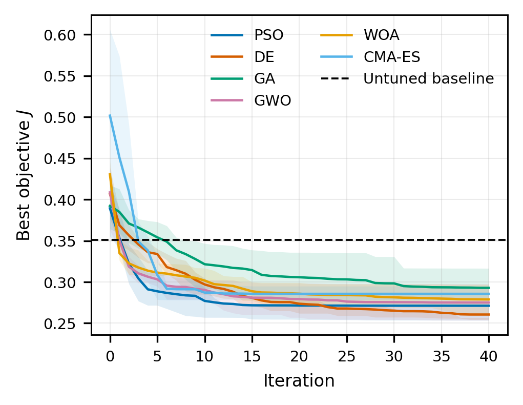
Figure 3. Convergence of the six optimisers over 40 iterations, mean of 10 runs with interquartile band. Dashed line: untuned analytic design
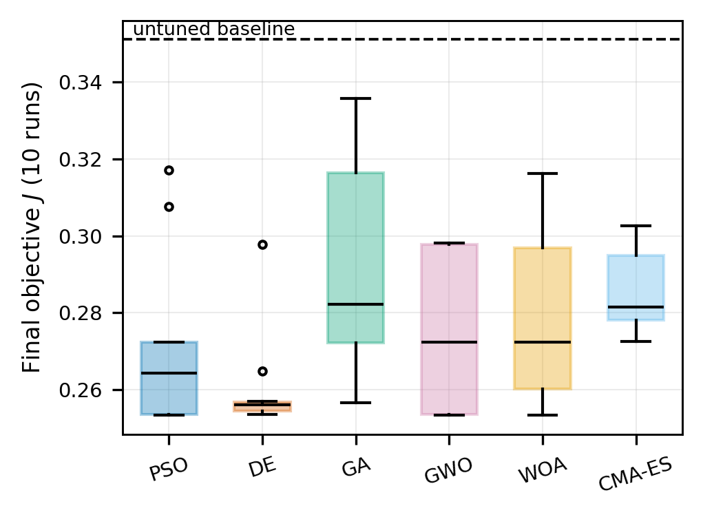
Figure 4. Distribution of the final objective over 10 independent runs per algorithm
Detection and Discrimination Performance
Table 6 compares the six tuned designs, the untuned analytic design and two baselines; Table 7 gives the per-family breakdown for the WOA-tuned design; Figure 5, Figure 6 and Figure 7 show representative residual traces, the discrimination map and the confusion matrix.
Three results are invariant across every tuned design. The false-alarm rate is zero in all 30 nominal runs (95 % upper bound 0.116), as Theorem 4 requires while disturbances and noise remain within their assumed bounds; Section 3.6 shows that it rises to 0.125 when the true disturbance exceeds the bound by 50 %. Channel attribution is 0.913–0.918, and the entire shortfall is attributable to one family, discussed below. Mean detection delay is 63–117 ms, that is, six to twelve samples.
No design dominates Table 6. The WOA-tuned design has the highest balanced accuracy (0.854), the highest MCC (0.696) and the shortest mean delay (63.3 ms), whereas the DE-tuned design has the highest TPR (0.874) and, in Table 5, the best mean objective. Table 7 and Figure 5 to Figure 7 use the WOA design. Because that choice was made on test-set metrics, they describe the best observed design rather than an independently selected one. A selection rule fixed in advance on a separate validation split would remove this bias and is recommended for future comparisons. The differences between the leading designs are small relative to their uncertainty: the TPR intervals of WOA (0.789–0.863) and DE (0.838–0.904) overlap, and a two-proportion test gives p = 0.065. For the WOA design, a bootstrap over runs stratified by family (5000 resamples) gives 95 % intervals of 0.840–0.868 for balanced accuracy and 0.666–0.725 for MCC.
Figure 5 shows the mechanism directly. Under loss of effectiveness and under command injection the actuation residual rises three to four orders of magnitude above its threshold within a few samples while the sensing residual stays flat; under a satellite-navigation bias fault the pattern is exactly reversed; and under telemetry forging the actuation residual remains at its noise floor while the sensing residual fires, which is Theorem 3 made visible.
Of the fourteen anomaly families, eleven are detected in every run and eight of these are also classified without error; the nominal class raises no alarm. Every actuation family is detected within 10 ms of onset and classified without error, and abrupt sensor faults are detected at the sample they occur, as predicted by the unit direct feedthrough. Three families are detected in every run but not always classified correctly: GNSS bias (0.67), sensor stuck (0.70) and gyro replay (0.97). Three are detected poorly or not at all: GNSS drift and GNSS spoofing (0 of 30 runs each) and oscillatory sensor injection (18 of 30). Excluding the two drift families, which lie below the drift bound of (14), the detection rate is 0.967 (348 of 360 runs).
The mean delay of 63.3 ms is an average over all 348 detected runs and is shaped by two families. Weighting each family’s mean delay by its detected runs gives (30 × 437 + 18 × 496)/348 = 63.3 ms, where 437 ms is the sum of the mean delays of the eleven fully detected families and 496 ms is the mean delay of oscillatory sensor injection. Eight families are detected within 10 ms, command oscillation and sensor stuck within 59 ms, command ramp at 269 ms and oscillatory sensor injection at 496 ms, so the mean understates the delay for slow and oscillatory anomalies and should be read alongside the per-family values of Table 7.
Tuning is not cosmetic. Balanced accuracy rises from 0.721 for the untuned analytic design to 0.854, and the Matthews correlation coefficient from 0.426 to 0.696 — a 63 % relative improvement on the metric least forgiving of class imbalance.
Figure 6 shows the actuation-channel verdicts in the ( ) plane. All actuation-fault runs lie at
 , well to the right of = 0.969, with
 between about −0.45 and 0 for loss of effectiveness and rotor offset and at = −1 for total rotor loss, inside the admissible set of (16). The large margin to ρthr shows that the classification as an actuation fault is not sensitive to the value of the threshold; that is, no attack run falls into the shaded region of the allowable space.
The residual confusion structure is given in Figure 7. None of the anomalous runs are assigned to the nominal class once they are detected and the remaining errors are 19 faults read as attacks (10 GNSS-bias and 9 sensor-stuck runs) against one attack read as a fault (one gyro-replay run). So the challenge is not so much detecting the faults, but distinguishing between them and attacks. Table 8 summarizes the consequences of the two types of errors: a fault read as an attack would make the vehicle distrust the channel and give up on the mission, while an attack read as a fault on the actuation channel would result in allocation computed based on commands sent by the attacker.
The fault-mimicking family behaves exactly as Theorem 5 predicts — 100 % detected, 100 % classified as fault. This is the theorem’s content, not a failure. Such an attack must confine itself to dissipative, affine, time-invariant behaviour, and the reallocation triggered by the fault verdict is the correct response to the trajectory it produces. For partial loss of effectiveness this response is adequate; for a mimicked total rotor loss it is the same emergency response that a real loss would require.
Table 6. All designs and comparison baselines on the 450-run test set. The last column gives the 95 % Clopper–Pearson interval for TPR over the 420 anomalous runs.
Design | TPR | FAR | Balanced acc. | Channel acc. | MCC | Mean delay (ms) | TPR 95 % CI |
PSO | 0.824 | 0.000 | 0.846 | 0.913 | 0.680 | 90.4 | 0.784–0.859 |
DE | 0.874 | 0.000 | 0.852 | 0.918 | 0.674 | 110.2 | 0.838–0.904 |
GA | 0.855 | 0.000 | 0.843 | 0.916 | 0.660 | 89.6 | 0.817–0.887 |
GWO | 0.833 | 0.000 | 0.816 | 0.914 | 0.612 | 117.5 | 0.794–0.868 |
WOA | 0.829 | 0.000 | 0.854 | 0.914 | 0.696 | 63.3 | 0.789–0.863 |
CMA-ES | 0.821 | 0.000 | 0.792 | 0.913 | 0.561 | 84.8 | 0.781–0.857 |
Untuned analytic | 0.786 | 0.000 | 0.721 | 0.909 | 0.426 | 92.6 | 0.743–0.824 |
B1 single observer | 0.829 | 0.000 | 0.670 | 0.943 | 0.269 | 123.1 | 0.789–0.863 |
B3 static telemetry | 0.429 | 0.000 | — | — | — | 35.7 | 0.381–0.477 |
Table 7. Per-family performance for the best design (WOA;  ,
 ,
 ). Values in parentheses are 95 % Clopper–Pearson intervals (30 runs per family).
Family | Detection rate | Classification accuracy | Channel accuracy | Mean delay (ms) |
Nominal | 0.00 (0.00–0.12) | 1.00 (0.88–1.00) | — | — |
Loss of effectiveness | 1.00 (0.88–1.00) | 1.00 (0.88–1.00) | 1.00 | 10 |
Rotor offset | 1.00 (0.88–1.00) | 1.00 (0.88–1.00) | 1.00 | 10 |
Total rotor loss | 1.00 (0.88–1.00) | 1.00 (0.88–1.00) | 1.00 | 10 |
Command step FDI | 1.00 (0.88–1.00) | 1.00 (0.88–1.00) | 1.00 | 10 |
Command oscillatory FDI | 1.00 (0.88–1.00) | 1.00 (0.88–1.00) | 1.00 | 59 |
Command ramp FDI | 1.00 (0.88–1.00) | 1.00 (0.88–1.00) | 1.00 | 269 |
Telemetry forging | 1.00 (0.88–1.00) | 1.00 (0.88–1.00) | 0.00 | 10 |
GNSS bias fault | 1.00 (0.88–1.00) | 0.67 (0.47–0.83) | 1.00 | 0 |
AHRS bias fault | 1.00 (0.88–1.00) | 1.00 (0.88–1.00) | 1.00 | 0 |
GNSS drift fault | 0.00 (0.00–0.12) | 0.00 (0.00–0.12) | — | — |
Sensor stuck fault | 1.00 (0.88–1.00) | 0.70 (0.51–0.85) | 1.00 | 59 |
GNSS spoofing | 0.00 (0.00–0.12) | 0.00 (0.00–0.12) | — | — |
Sensor oscillatory FDI | 0.60 (0.41–0.77) | 0.60 (0.41–0.77) | 1.00 | 496 |
Gyro replay | 1.00 (0.88–1.00) | 0.97 (0.83–1.00) | 1.00 | 0 |
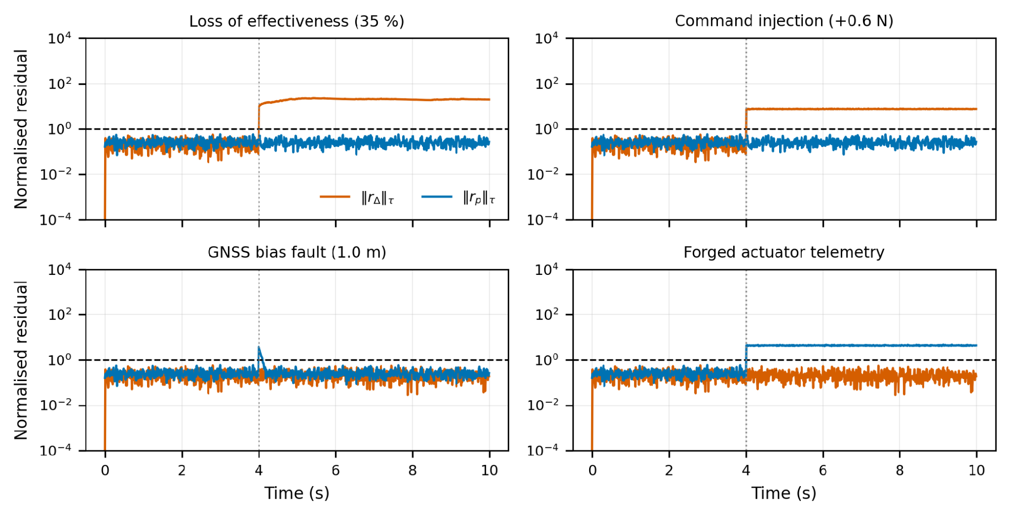
Figure 5. Normalised residuals for four representative anomalies, onset at 4 s. Dashed line marks the detection threshold
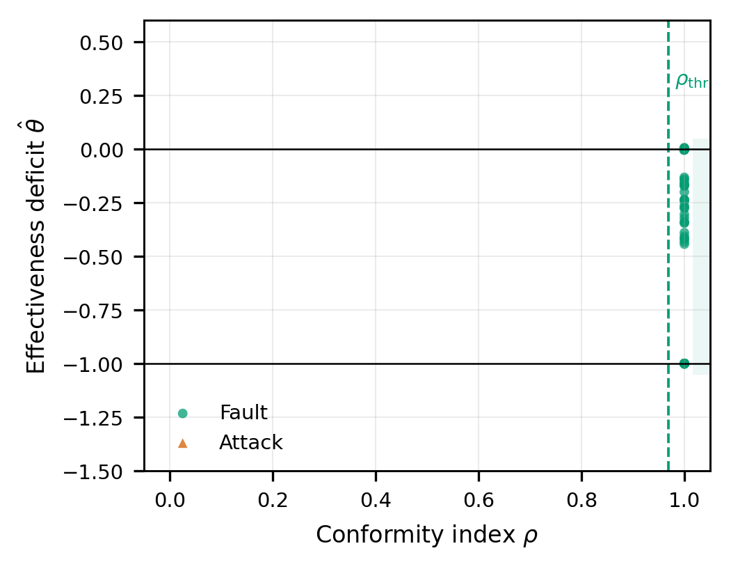
Figure 6. Actuation-channel discrimination in the  plane
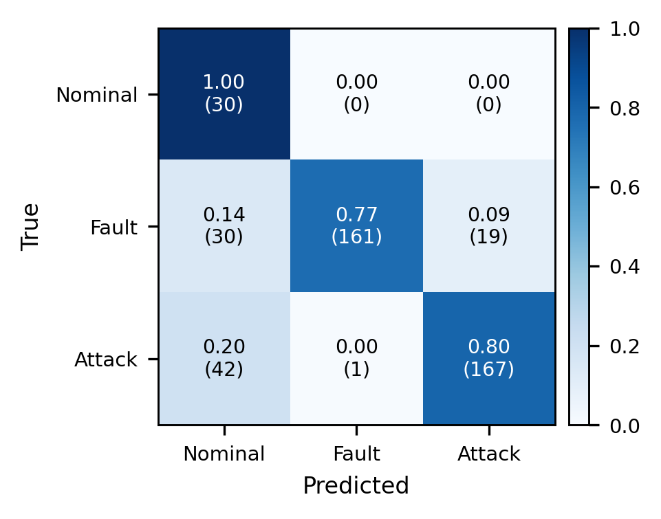
Figure 7. Confusion matrix for the tuned design over 450 Monte Carlo runs; row-normalised, counts in parentheses
Table 8. Verdicts of the WOA-tuned design (Figure 7) and the response each verdict triggers.
True Class | Verdict | Runs | Intended Response | Consequence |
Nominal | Nominal | 30 | None | Correct |
Fault | Fault | 161 | Reallocate thrust (actuation) or isolate the faulty unit (sensing) | Correct; the mission can continue |
Fault | Attack | 19 (10 GNSS bias, 9 sensor stuck) | Distrust the channel; hold, land or return | Mission abandoned unnecessarily; vehicle preserved |
Fault | Nominal (missed) | 30 (GNSS drift) | None | Navigation error grows undetected |
Attack | Attack | 167 | Distrust the channel; hold, land or return | Correct |
Attack | Fault | 1 (gyro replay) | Isolate the gyro as a faulty unit | Replayed signal removed; outcome close to the attack response |
Attack | Nominal (missed) | 42 (30 GNSS spoofing, 12 oscillatory injection) | None | Adversary keeps influence on navigation |
Validation of the Guaranteed Bounds
Table 9 and Figure 8 compare each bound of Theorem 4 with the smallest tested anomaly magnitude at which every Monte Carlo run detected the anomaly.
Figure 8 and Table 9 compare each bound against Monte Carlo detection probability. In every case detection occurs earlier than promised and never later, which is the correct behaviour for a sufficient condition: the bounds are worst-case over noise realisations and anomaly directions, whereas the Monte Carlo samples typical ones. A bound that were tight would necessarily be violated on unfavourable realisations, and the zero-false-alarm guarantee would fail with it. The conservatism factors of 1.7 to 3.2 quantify the price of that safety and are, we would argue, acceptable: a factor of two on the minimum detectable fault is a small cost for a false-alarm rate that is zero by construction rather than by tuning.
Two qualifications apply. First, the empirical values are grid points: for GNSS drift, detection is zero at 2 m/s and complete at the next grid point, 8.0 m/s, so the true threshold lies between the two and the conservatism factor of 3.2 is an upper estimate. Second, complete detection in a finite number of runs is not a detection probability of one: with n runs all detected, the 95 % Clopper–Pearson lower bound is  , which is 0.88 for
 = 30.
The identifiability law (19) is tested next by varying the excitation index of the command dither Figure 9. Figure 9 tests the identifiability law (19). Above  the empirical standard deviation of tracks the prediction closely — 0.00065 against 0.00051 at
 — confirming the inverse-square-root scaling. Below that the empirical value exceeds prediction by roughly threefold and is non-monotone. The discrepancy is real, and we attribute it to error sources (19) does not model: window transients following the alarm, and brief actuator saturation during aggressive segments of the reference. The law should therefore be read as an asymptotic floor on achievable precision rather than an exact predictor at low excitation.
Table 9. Theoretical bounds against empirical thresholds for complete detection. The drift rate is the rate at which the injected error in the reported GNSS position grows; it is not a motion of the airframe.
Anomaly Class | Guaranteed Bound (Theory) | Empirical 100 % Detection | Conservatism Factor |
Actuation anomaly (per rotor) | 5.17 % LoE | 2.00 % LoE | 2.6 |
Abrupt sensing anomaly (GNSS) | 0.522 m | 0.30 m | 1.7 |
Sensing drift rate (GNSS) | 25.9 m/s | 8.0 m/s | 3.2 |
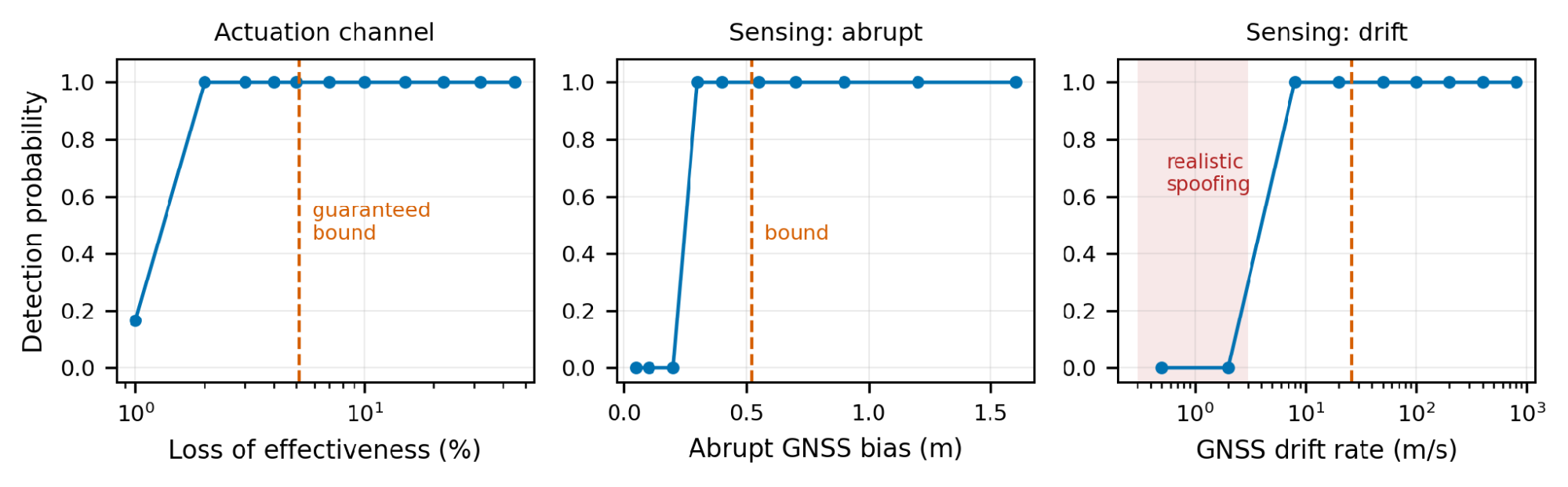
Figure 8. Detection probability against anomaly magnitude for the three anomaly classes, with the guaranteed bounds of Theorem 4 marked. Shaded band: realistic spoofing rates
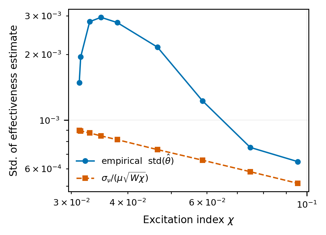
Figure 9. Empirical standard deviation of the effectiveness estimate against excitation index, compared with the identifiability law of (19)
Ablation and Comparison with Alternative Architectures
Each of the structural options is isolated by three baselines for comparison Figure 10 and is summarised per-family in Table 7, which also includes the result of the per-family detection.
B1 — single command-anchored observer using a structured-residual dictionary test (classical model-based diagnosis). It achieves the same rate of detection (0.829) as well as the same number of zero false alarms, and even improves the fit of the channel slightly (0.943), since it estimates the forging attack to the actuation dictionary directly. But its balanced accuracy is 0.670 against 0.854 and its MCC 0.269 against 0.696. The reason is structural, because the one residual, the anomaly in the actuator and the anomaly in the sensor are overlapping, and thus, the type of anomaly has to be determined by the shape of the residual only and the argument of dissipativity of (16) cannot be used at all. The hard part isn't detecting, it's discrimination! This comparison is the most explicit claim of contribution of the paper.
A — good twin observers (matched gains), testing Theorem 2.Theorems 2 and 3 are tested for the twins A and B, respectively. When the normalised  is triggered with the anomaly, it is 4×
 times above its threshold, and the false channel attribution rate is 100 %. The leakage term in (10) is not just a cause of degradation of decoupling, but it is the cause of its destruction. Gain matching is a load bearing method.
B3 — static comparison 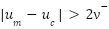 , to check if the observer pair is required at all on the actuation channel. It has 0 detection with zero false alarm and is totally blind to the telemetry-forging family, which is 100 % detected by Theorem 3 for all the runs. The static test is a sound, but not necessarily adaptive, test of actuation-integrity.
The one thing that remained a mystery in the channel-attribution numbers is now made sense of. The sensing channel is responsible for telemetry forging in 100 % of runs, resulting in an aggregate channel accuracy of 0.914 which is exactly what Theorem 3 predicts. The actual signature that is left is the sensing channel, and the physical source is the actuation path. The classification is valid: 100 % attack, as the residual passes through B_d and the sensor dictionary (20) is not able to fit it. Labelling this as an “attribution error” is an artefact, and we prefer that to be revealed rather than modeled after to “flatter the result.”
The pattern can be seen in Figure 10. The TPR (0.79–0.83) and channel accuracy (0.91–0.94) of tuned and untuned dual-residual designs and B1 are comparable; however, their balanced accuracy and MCC scores are distinctively separated (0.696, 0.426 and 0.269) and B3 detects only 0.429 of the anomalous runs.
Read together, the three ablations test the mechanism rather than add performance comparisons: B1 shows that discrimination requires access to δu, which only the dual structure provides; B2 confirms the necessity statement of Theorem 2; and B3 confirms the coverage statement of Theorem 3.
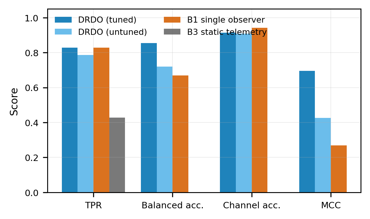
Figure 10. Tuned dual-residual observer against untuned design and two alternative designs
Robustness
Figure 11 tests the assumptions underlying Theorem 4 by letting the true disturbance and noise exceed the bounds used in design by a factor  .
Figure 11 shows sensitivity to the assumptions underlying Theorem 4. Varying wind and noise scaling within the assumed bounds leaves the false-alarm rate at zero and balanced accuracy between 0.810 and 0.833, as the theorem requires. The informative experiment is bound violation: allowing the true disturbance and noise to exceed their design bounds by a factor . At  the false-alarm rate remains exactly zero; at
 it is 0.125; at
 it is 1.000 and balanced accuracy collapses to 0.369.
The guarantee is thus not brittle at its boundary — roughly 25 % under-estimation of the disturbance envelope is tolerated in practice, because the peak-gain bound is itself conservative — but it degrades sharply beyond that. Identifying the envelope conservatively is the single most important practical requirement of the method, and an operator who sets from fair-weather flight data will get false alarms in gusts.
Plant-model mismatch. The two residuals respond differently to modelling errors. Because both observers use the same matrices, the cancellation in Theorem 1 does not depend on the true plant: errors in mass, inertia, arm length or drag cannot leak into , although they change the closed-loop trajectory and hence uc. They do enter , as the unmodelled input  in the error dynamics (11), where the subscript 0 marks the nominal model used by the observers, and they can therefore cause sensing-channel false alarms unless is enlarged by a corresponding bound. The one modelling error that reaches rΔ is actuator dynamics: a motor with time constant
 delivers thrust that lags the command, so
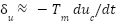 during nominal transients. The actuation threshold must then cover times the largest commanded thrust rate, or observer 1 must be driven by a nominal actuator model
 instead of .
These effects are established analytically here. A Monte Carlo evaluation with perturbed mass, inertia, rotor coefficients and motor lag has not been carried out in the present study and is listed among the limitations in Section 3.7.4.
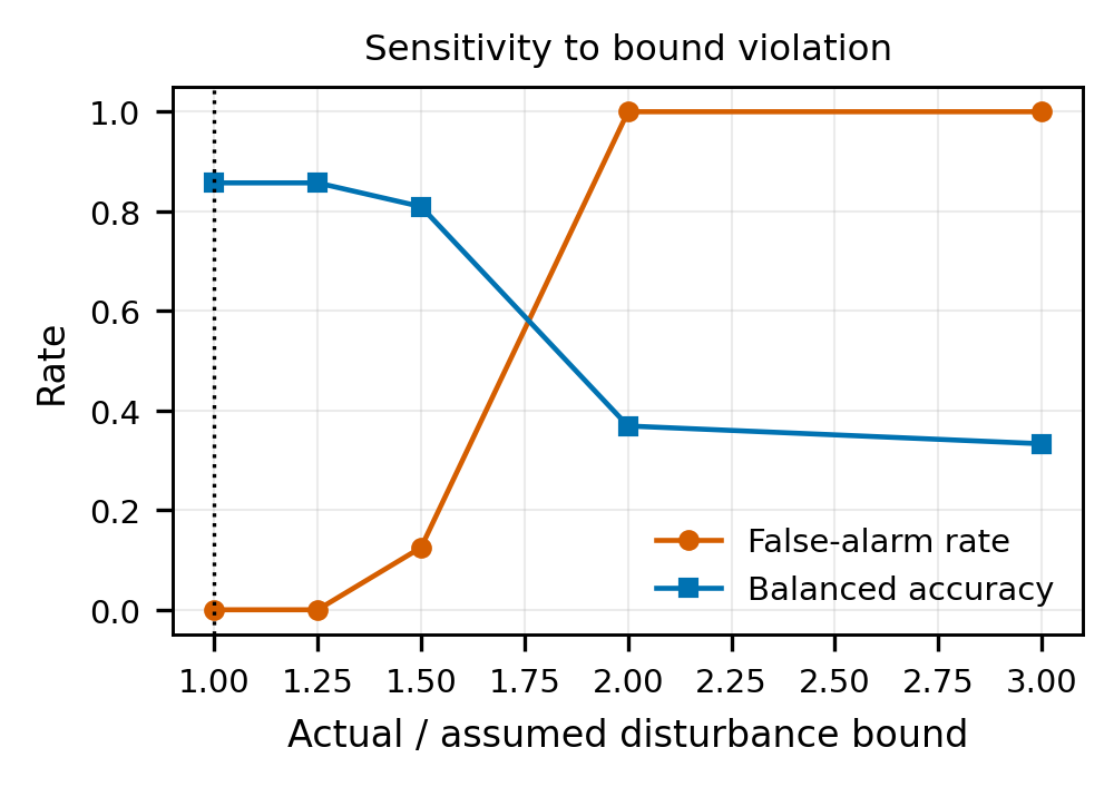
Figure 11. False-alarm rate and balanced accuracy as the true disturbance and noise exceed their assumed bounds by a factor
Discussion
Main Findings
Three findings stand out. First, detection is not the difficulty; discrimination is. The single-observer baseline matches the proposed design on TPR (0.829) and false alarms, but its MCC is 0.269 against 0.696, and the residual confusion of Figure 7 lies between faults and attacks rather than between anomalous and nominal runs. Second, the separation is structural: mismatched gains destroy it, with leakage of 4 × times the threshold, and forged telemetry is exposed on the second residual in every run, as Theorem 3 predicts. Third, the guarantees hold only under their assumptions: there are no false alarms within the disturbance bounds but a rate of 0.125 at 1.5 times the bound, and slow GNSS drift and spoofing are not detected at all.
Comparison with Other Studies
Against the observer-based fault-tolerant control literature [9]–[11],[13]–[15], the present scheme adds an admissibility test that those designs do not perform: they reconstruct an anomaly and feed it to reallocation without asking whether hardware could have produced it. Our results indicate the cost of that omission is not detection performance — B1 matches us on detection — but the misdirection of the reconfiguration response, which is the outcome the security literature warns about [1],[5]. Set-based observers [16]–[19] share the present emphasis on guaranteed thresholds and minimum detectable faults; they address faults only, whereas here a bound of the same kind is combined with a fault-versus-attack test.
Against learning-based UAV attack and fault detection, the difference is the nature of the guarantee (Table 10). Those methods report accuracies of 98–99.8 % on labelled data for a single anomaly class, GNSS spoofing [26][27],[32] or complete actuator failure [21], and, where reported, an empirical false-alarm rate of 3 % [27]. The present design addresses fourteen fault and attack families at once and reports a false-alarm rate that is zero by construction under stated bounds and detection thresholds in closed form, at the price of a linearised model, stated noise envelopes and lower per-class accuracy. Because data, vehicles and anomaly sets differ, the figures in Table 10 are not directly comparable. The two approaches are complements rather than competitors: learning-based spoofing detectors succeed exactly where (14) shows a fixed-threshold residual test must fail, and a data-driven layer of the kind used in [21][22] is the natural way to attack the drift regime.
Against the cyber-physical security literature [39][40],[43],[47], the distinguishing feature is that we exploit a structural asymmetry specific to aerial vehicles. Secure state estimation for general plants must reason about which measurement subsets are trustworthy, because actuation and sensing are not separable. A multirotor carries actuator-side telemetry, and Theorems 1 and 3 convert that redundancy into an exact partition of the anomaly space. The closest discrimination methods [50]–[52] achieve separation through distributed decoupling, watermarking or coding; the present method needs no injected signal but relies on actuator telemetry and leaves a characterised set of mimicking attacks. The stealthy-attack constructions of [47] remain relevant, however, and our drift limitation is precisely an instance of them.
The value of a deterministic threshold is easiest to see against a statistical one. A chi-square test on Kalman-filter innovations with a per-sample false-alarm probability of , run at 100 Hz, raises at least one false alarm during a 10 s flight with probability  ; the peak-gain thresholds of (12) raise none while the bounds hold. The price is the conservatism quantified in Table 9.
Table 10. Results reported by representative studies and by the present work. Data, vehicles and anomaly sets differ, so the figures are not directly comparable
Study | Task | Data | Reported Result | Fault vs Attack | False-Alarm Figure |
Ma et al. [26] | GNSS spoofing detection (stacked ensemble) | Flight data, Pixhawk 4 receiver, SDR-generated spoofing | Accuracy 99.79 % | No | Not reported |
Alhoraibi et al. [27] | GNSS spoofing detection (adversarial ML) | Eight-channel receiver data, 510 530 samples | Accuracy 98 % | No | 3 % (empirical) |
Sun et al. [32] | GNSS spoofing detection (PCA-CNN-LSTM) | GPS-signal data set from a small UAV and a spoofing jammer | Accuracy 99.49 % | No | Not reported |
Debele et al. [21] | Actuator fault detection and isolation (cascaded deep networks) | 16-rotor UAV, complete actuator failure | Accuracy 98.97 % (region), 99.107 % (rotor) | No | Not reported |
B1 single observer (this study) | Detection and classification | 450 simulated runs, 14 families | TPR 0.829; BA 0.670; MCC 0.269 | Partly | 0 under bounds |
Proposed (this study) | Detection, channel attribution and classification | 450 simulated runs, 14 families | TPR 0.829; BA 0.854; MCC 0.696 | Yes | 0 under bounds (deterministic); 0.125 at 1.5× bound |
Implications and Explanation of Findings
Coverage gaps define where the method can be trusted. Slow GNSS drift and GNSS spoofing at 0.8–2.5 m/s were never detected (0 of 30 runs each; 95 % upper bound 0.12). The cause is purely structural: a constant observer bias gets integrated into the observer state estimate at a slow rate, and the drift bound of (14) is 25.9 m/s. From an operational perspective, a spoofer with a drift rate of 2 m/s would be able to misestimate the position by 120 m during 1 minute without raising an alarm. Operationally, a spoofer drifting at 2 m/s could displace the position estimate by 120 m within one minute without an alarm. Oscillatory sensor injection was detected in 18 of 30 runs (95 % interval 0.41–0.77) with a 496 ms mean delay, because its frequency content falls where the tuned observer is least sensitive. The method therefore cannot secure satellite navigation on its own; it must be paired with an independent position source, with gain modulation, or with a learning-based spoofing detector of the kind listed in Table 10.
The 19 fault was an attack on availability – that is, the vehicle would drop a mission it could have accomplished. A replay of a single attack faulted as a fault was a gyro replay, where isolating the gyro eliminates the replayed signal. An attack read as a fault on the actuation channel would cause reallocation to follow the adversary's command, and this error did not occur in the test set; however, Theorem 5 implies that an adversary with a fault would cause such a fault.
The reliance on actuator telemetry is a scheme's power and primary practical requirement. The accuracy of telemetry is used to set the actuation detection limit, but a speed-only telemetry also allows propeller damage to fall outside the actuation channel Section 2.2.
Strengths and Limitations
Strengths. The separation of the actuation and sensing path is proved instead of learned; the guarantee of a false alarm, and the detection bounds are explicitly stated and were not violated in simulation, within the bounds of the assumptions; the blind spots are stated as bounds, not discovered in service; and the runtime cost is approximately 708 operations per sample. The limitations follow.
Provably slow sensor drift is undetectable. Table 7 shows that no runs were detected as realistic satellite-navigation spoofing (0 % of runs) when the spoof velocity was set to 0.8–2.5 m . From (14) follows this that, when the bias on the sensor is slowly varying, the steady state observer will incorporate it into its state estimate and thus reduce the DC sensitivity to zero. The optimiser reduced it by about ten times, compared to the untuned design, the bound was raised from over 130 m to 25.9 m., but it could not eliminate it entirely, as the bound is structural and not parametric. Future work: sub-bound detection requires information outside the modelled sensor set; the natural routes are an independent positioning modality or randomised gain modulation, which makes the DC null non-stationary so that a constant-rate drift produces a detectable transient at each switch.
The indistinguishable set is non-empty. By Theorem 5, a dissipative attack that is affine in the command with constant coefficients cannot be separated from a passive fault, as confirmed by the fault-mimicking family. The vehicle then responds as it would to the equivalent fault, which is adequate for partial loss of effectiveness but, for a mimicked total rotor loss on a quadrotor, forces an emergency; an adversary aware of the constraint can operate within it indefinitely. Future work: narrowing the set requires independent authentication of the command path — a cryptographic rather than an observer-theoretic remedy.
The guarantee inherits its assumptions. Zero false alarms hold only while the disturbance and noise respect their assumed envelopes; Section 3.6 measured the failure at  . Future work: an online envelope estimator that adapts to observed gust statistics, at the cost of replacing the deterministic guarantee with a high-probability one.
Actuator-side telemetry is required. The architecture presumes measured rotor thrust from electronic-speed-controller feedback; vehicles without it cannot form . Future work: substituting an inertial-derived thrust estimate would preserve the structure at the cost of Theorem 1’s exactness.
Propeller damage may bypass the actuation channel. With thrust derived from rotor speed alone, a damaged propeller lowers thrust without changing speed, so the anomaly appears on rather than and may be labelled an attack. Future work: motor-current telemetry and a powertrain model [25] would return such damage to the actuation channel, and this case should be evaluated explicitly.
Fault classes outside the model. Intermittent faults violate time invariance and ESC runaway violates dissipativity, so both would be labelled attacks; neither was included in the test set. Future work: extend the admissible set to switching or slowly varying parameters and evaluate both cases.
Robustness to model mismatch is analysed but not yet measured. Section 3.6 shows which residual each modelling error reaches, but the size of the effect has not been simulated, so the zero-false-alarm guarantee is untested under plant-model mismatch. Future work: a Monte Carlo study with perturbed mass, inertia, rotor coefficients and motor lag, enlarging by a mismatch bound where needed.
Marginal sensor anomalies classify poorly. GNSS bias and stuck-sensor families classify at 0.67 and 0.70 Table 7, because anomalies close to the detection threshold produce signatures whose energy is comparable to the disturbance within the fitting window. Future work: an adaptive window that trades verdict latency against fit quality, triggered by the observed signal-to-threshold ratio.
This is partially detected using oscillatory sensor injection. The mean detection time for that family is 496 ms, with a detection of 0.60, as it has a frequency content that is not at the peak of the tuned observer's sensitivity. Future work: a multi-model observer bank in complementary frequency bands.
Validation is simulation only and linearised. The model describes a hover linearisation, and is linear with a linear mixer, which means it is valid in the vicinity of hover, but does not model aggressive manoeuvring, aerodynamic coupling and rotor dynamics. Future work: the bounded-envelope assumption on which the whole guarantee is based, must be tested on a vehicle with ESC telemetry, through hardware-in-the-loop and flight validation.
CONCLUSIONS
This paper aimed to make fault vs. attack a structural property of the observer, instead of an inference drawn from data. For two Luenberger observers designed by commanded and by measured thrust of the rotors they create a residual difference that is precisely invariant to all the signals traversed by the sensor, and depends only on the difference in the actuation. Gain matching is necessary and sufficient, and if an adversary silences the first via actuator telemetry, the second would be excited, and so the two cover the actuation path within the threat model of Section 2.2. In each of the channels, the discrimination is based on physical admissibility, and the attacks which can't be distinguished from faults are characterised exactly but in a way that isn't left implicit.
In Monte Carlo simulation of a quadrotor linearised about hover, the WOA-tuned design raised no false alarms while disturbances and noise stayed within their assumed bounds, detected 82.9 % of anomalous runs with a mean delay of 63 ms, and classified faults against attacks with 0.854 balanced accuracy (95 % interval 0.840–0.868) and 0.696 MCC, against 0.670 and 0.269 for a single-observer baseline. These guarantees are conditional: the false-alarm rate reached 0.125 when the disturbance exceeded its bound by 50 %. Eleven of fourteen anomaly families were detected in every run and eight were also classified without error, but slow GNSS drift and spoofing were never detected, and oscillatory sensor injection was detected in 60 % of runs. Similar final objective values across six optimisers indicate a similar solution region, not a proven global optimum; DE was the most reliable single-run choice.
Hardware-in-the-loop and flight validation on a vehicle with ESC telemetry is the essential next step and is required before any operational claim. Further priorities are extending the decoupling proof to linear-parameter-varying and nonlinear models, detecting slow drift through an independent position source or randomised gain modulation, using motor-current telemetry to bring propeller damage into the actuation channel, and evaluating the method under plant-model mismatch, on real actuator and sensor fault data and against adaptive stealthy attacks.
The complete simulation code, the generated figures and the tabulated experimental record accompany this manuscript and are available from the corresponding author on reasonable request. All results are reproducible from fixed random seeds using the scripts described in Section 2.8.
ABBREVIATIONS
The following abbreviations are used in this manuscript.
UAV | : | Unmanned Aerial Vehicle |
DRDO | : | Dual-Residual Diagnostic Observer |
FDI | : | False Data Injection |
LoE | : | Loss of Effectiveness |
GNSS | : | Global Navigation Satellite System |
AHRS | : | Attitude and Heading Reference System |
MDA | : | Minimum Detectable Actuation anomaly |
MDR | : | Minimum Detectable drift Rate |
FCI | : | Fault-model Conformity Index |
MCC | : | Matthews Correlation Coefficient |
ESC | : | Electronic Speed Controller |
TPR | : | True-Positive Rate |
FAR | : | False-Alarm Rate |
LPV | : | Linear Parameter-Varying |
PSO | : | Particle Swarm Optimisation |
DE | : | Differential Evolution |
GA | : | Genetic Algorithm |
GWO | : | Grey Wolf Optimiser |
WOA | : | Whale Optimization Algorithm |
CMA-ES | : | Covariance Matrix Adaptation Evolution Strategy |
REFERENCES
- J. Burbank, T. Caleb, E. Andam, and N. Kaabouch, “Detection and mitigation of cyber attacks on UAV networks,” Electronics, vol. 15, no. 2, p. 317, 2026, https://doi.org/10.3390/electronics15020317.
- K. Osmani and D. Schulz, “Comprehensive investigation of unmanned aerial vehicles (UAVs): An in-depth analysis of avionics systems,” Sensors, vol. 24, no. 10, p. 3064, 2024, https://doi.org/10.3390/s24103064.
- M. E. Yiğit, E. Bektaş, F. Korkmaz, and M. Teke, “Hybrid PSO MRFO optimization of PID parameters for real-time PMDC motor speed control,” Ain Shams Eng. J., vol. 17, no. 7, p. 104232, 2026, https://doi.org/10.1016/j.asej.2026.104232.
- E. Bektaş and H. Karaca, “GA based selective harmonic elimination for multilevel inverter with reduced number of switches: An experimental study,” Elektron. Elektrotech., vol. 25, no. 3, pp. 10–17, 2019, https://doi.org/10.5755/j01.eie.25.3.23670.
- E. Bektaş and H. Karaca, “GA based selective harmonic elimination for five level inverter using cascaded H bridge modules,” Int. J. Intell. Syst. Appl. Eng., vol. 4, no. 2, pp. 29–32, 2016, https://doi.org/10.18201/ijisae.97681.
- B. Graziano and A. Sargolzaei, “Cybersecurity of unmanned aerial vehicles from a control systems perspective: A review,” Electronics, vol. 15, no. 1, p. 163, 2026, https://doi.org/10.3390/electronics15010163.
- A. A. Alquwayzani and A. A. Albuali, “A systematic literature review of zero trust architecture for military UAV security systems,” IEEE Access, vol. 12, pp. 176033–176056, 2024, https://doi.org/10.1109/ACCESS.2024.3503587.
- S. Kim, K.-J. Park, and C. Lu, “A survey on network security for cyber–physical systems: From threats to resilient design,” IEEE Commun. Surv. Tutor., vol. 24, no. 3, pp. 1534–1573, 2022, https://doi.org/10.1109/COMST.2022.3187531.
- X. Hu, B. Wang, Y. Shen, Y. Fu, and N. Li, “Disturbance observer-enhanced adaptive fault-tolerant control of a quadrotor UAV against actuator faults and disturbances,” Drones, vol. 7, no. 8, p. 541, 2023, https://doi.org/10.3390/drones7080541.
- S. A. Ahmed et al., “Advancements in UAV image semantic segmentation: A comprehensive literature review,” Multidiscip. Rev., vol. 7, no. 6, p. 2024118, 2024, https://doi.org/10.31893/multirev.2024118.
- S. A. Ahmed, H. Desa, A.-S. T. Hussain, and T. A. Taha, “Implementation of deep neural networks learning on unmanned aerial vehicle based remote-sensing,” IAES Int. J. Artif. Intell., vol. 13, no. 1, pp. 941–947, 2024, https://doi.org/10.11591/ijai.v13.i1.pp941-947.
- S. A. Ahmed, H. Desa, and A.-S. T. Hussain, “Aerial image semantic segmentation based on 3D fits a small dataset of 1D,” IAES Int. J. Artif. Intell., vol. 12, no. 4, pp. 2048–2054, 2023, https://doi.org/10.11591/ijai.v12.i4.pp2048-2054.
- S. A. Ahmed, H. Desa, and A.-S. T. Hussain, “Classification of semantic segmentation using fully convolutional networks based unmanned aerial vehicle application,” IAES Int. J. Artif. Intell., vol. 12, no. 2, pp. 641–647, 2023, https://doi.org/10.11591/ijai.v12.i2.pp641-647.
- R. Zheng, Q. Zhu, S. Huang, Z. Du, J. Shi, and Y. Lyu, “Extended state observer-based sliding-mode control for aircraft in tight formation considering wake vortices and uncertainty,” Drones, vol. 8, no. 4, p. 165, 2024, https://doi.org/10.3390/drones8040165.
- Y. Jing, A. Mirza, R. Sipahi, and J. Martinez-Lorenzo, “Sliding mode controller with disturbance observer for quadcopters; experiments with dynamic disturbances and in turbulent indoor space,” Drones, vol. 7, no. 5, p. 328, 2023, https://doi.org/10.3390/drones7050328.
- X. Zhu, Y. Li, G. Yin, and R. J. Patton, “Interval observer-based fault detection and isolation for quadrotor UAV with cable-suspended load,” IEEE Trans. Syst., Man, Cybern., Syst., vol. 54, no. 10, pp. 5876–5888, 2024, https://doi.org/10.1109/TSMC.2024.3411315.
- J. Li, Y. Liu, Y. Jiang, Z. Wang, and Y. Li, “Fault detection for autonomous underwater vehicles based on zonotopic set-membership estimation,” IEEE Trans. Ind. Inform., vol. 21, no. 11, pp. 8453–8462, 2025, https://doi.org/10.1109/TII.2025.3582373.
- Z. Wang, C. Xu, Z. Liu, and Y. Shen, “Fault detection for satellite reaction wheel based on zonotopic set-membership estimation,” IEEE Trans. Aerosp. Electron. Syst., vol. 61, no. 2, pp. 1577–1588, 2025, https://doi.org/10.1109/TAES.2024.3457745.
- S. Zhang, V. Puig, and S. Ifqir, “Robust LPV fault diagnosis using the set-based approach for autonomous ground vehicles,” IEEE Trans. Intell. Transp. Syst., vol. 25, no. 8, pp. 9078–9090, 2024, https://doi.org/10.1109/TITS.2024.3394518.
- J. D. Lee, S. Im, L. Kim, H. Ahn, and H. Bang, “Data-driven fault detection and isolation for multirotor system using Koopman operator,” J. Intell. Robot. Syst., vol. 110, p. 128, 2024, https://doi.org/10.1007/s10846-024-02142-y.
- Y. Debele, H.-Y. Shi, A. Wondosen, T.-W. Ku, and B.-S. Kang, “Deep learning-based robust actuator fault detection and isolation scheme for highly redundant multirotor UAVs,” Drones, vol. 7, no. 7, p. 437, 2023, https://doi.org/10.3390/drones7070437.
- N. Liu, Z. Zhou, L. Zhu, Y. He, and F. Huang, “Fault diagnosis of unmanned aerial systems using the Dempster–Shafer evidence theory,” Actuators, vol. 13, no. 7, p. 264, 2024, https://doi.org/10.3390/act13070264.
- W. Wen, W. Zhong, Y. Liu, X. Li, and H. Lan, “Fault diagnosis of UAV rotor systems based on drone nest vibration analysis,” Drones, vol. 10, no. 6, p. 424, 2026, https://doi.org/10.3390/drones10060424.
- A. Baldini, R. Felicetti, F. Ferracuti, A. Freddi, S. Iarlori, and A. Monteriù, “Real-time propeller fault detection for multirotor drones based on vibration data analysis,” Eng. Appl. Artif. Intell., vol. 123, p. 106343, 2023, https://doi.org/10.1016/j.engappai.2023.106343.
- A. Baldini, R. Felicetti, F. Ferracuti, A. Freddi, and A. Monteriù, “Propeller fault detection and isolation for multirotor drones with adaptation to battery voltage drop,” J. Intell. Robot. Syst., vol. 112, p. 28, 2026, https://doi.org/10.1007/s10846-026-02369-x.
- T. Ma, X. Zhang, and Z. Miao, “Detection of UAV GPS spoofing attacks using a stacked ensemble method,” Drones, vol. 9, no. 1, p. 2, 2025, https://doi.org/10.3390/drones9010002.
- L. Alhoraibi, D. Alghazzawi, and R. Alhebshi, “Detection of GPS spoofing attacks in UAVs based on adversarial machine learning model,” Sensors, vol. 24, no. 18, p. 6156, 2024, https://doi.org/10.3390/s24186156.
- R. Al-Syouf, O. Y. Aljarrah, R. Bani-Hani, and A. Alma’aitah, “Ensemble machine learning models utilizing a hybrid recursive feature elimination (RFE) technique for detecting GPS spoofing attacks against unmanned aerial vehicles,” Sensors, vol. 25, no. 8, p. 2388, 2025, https://doi.org/10.3390/s25082388.
- M. Mouzai, M. A. Riahla, A. Keziou, and H. Fouchal, “Exploring multi-channel GPS receivers for detecting spoofing attacks on UAVs using machine learning,” Sensors, vol. 25, no. 13, p. 4045, 2025, https://doi.org/10.3390/s25134045.
- K. Radoš, M. Brkić, and D. Begušić, “Recent advances on jamming and spoofing detection in GNSS,” Sensors, vol. 24, no. 13, p. 4210, 2024, https://doi.org/10.3390/s24134210.
- A. Mohanty and G. Gao, “A survey of machine learning techniques for improving Global Navigation Satellite Systems,” EURASIP J. Adv. Signal Process., vol. 2024, p. 73, 2024, https://doi.org/10.1186/s13634-024-01167-7.
- Y. Sun, M. Yu, L. Wang, T. Li, and M. Dong, “A deep-learning-based GPS signal spoofing detection method for small UAVs,” Drones, vol. 7, no. 6, p. 370, 2023, https://doi.org/10.3390/drones7060370.
- G. Wang, J. Ai, L. Mo, X. Yi, P. Wu, X. Wu, and L. Kong, “Anomaly detection for data from unmanned systems via improved graph neural networks with attention mechanism,” Drones, vol. 7, no. 5, p. 326, 2023, https://doi.org/10.3390/drones7050326.
- H. Khazane, M. Ridouani, F. Salahdine, and N. Kaabouch, “A holistic review of machine learning adversarial attacks in IoT networks,” Future Internet, vol. 16, no. 1, p. 32, 2024, https://doi.org/10.3390/fi16010032.
- T. Talaei Khoei and N. Kaabouch, “A comparative analysis of supervised and unsupervised models for detecting attacks on the intrusion detection systems,” Information, vol. 14, no. 2, p. 103, 2023, https://doi.org/10.3390/info14020103.
- K. Pan, Y. Lyu, F. Yang, Z. Tan, and Q. Pan, “Attack detection and security control for UAVs against attacks on desired trajectory,” J. Intell. Robot. Syst., vol. 110, p. 68, 2024, https://doi.org/10.1007/s10846-024-02086-3.
- K. Pan, F. Yang, Y. Lyu, M. Ji, and Q. Pan, “Neural observer-based formation for multi-UAVs against deception and desired trajectory attacks,” Neurocomputing, vol. 622, p. 129297, 2025, https://doi.org/10.1016/j.neucom.2024.129297.
- M.-Y. Lee, H. Chiu, and B.-S. Chen, “Networked security observer-based reference tracking control of stochastic quadrotor UAV system under cyber-attack: T-S fuzzy approach,” IEEE Access, vol. 10, pp. 30296–30322, 2022, https://doi.org/10.1109/ACCESS.2022.3158345.
- W. Xing and J. Shen, “Security control of cyber–physical systems under cyber attacks: A survey,” Sensors, vol. 24, no. 12, p. 3815, 2024, https://doi.org/10.3390/s24123815.
- D. Ding, Q.-L. Han, X. Ge, and J. Wang, “Secure state estimation and control of cyber-physical systems: A survey,” IEEE Trans. Syst., Man, Cybern., Syst., vol. 51, no. 1, pp. 176–190, 2021, https://doi.org/10.1109/TSMC.2020.3041121.
- Y. K. Shi, Y. Q. Wang, and J. Y. Tuo, “Distributed secure state estimation of multi-agent systems under homologous sensor attacks,” IEEE/CAA J. Autom. Sinica, vol. 10, no. 1, pp. 67–77, 2023, https://doi.org/10.1109/JAS.2022.105920.
- X. Feng, X. Li, S. Li, and F. Pan, “Secure state estimation for unmanned aircraft cyber-physical systems under multiple attacks,” Asian J. Control, vol. 24, no. 2, pp. 818–833, 2022, https://doi.org/10.1002/asjc.2757.
- L. Xu, Y. Zhu, Z. Li, and Q. Zhang, “Safety control for cyber–physical systems under false data injection attacks,” Electronics, vol. 14, no. 6, p. 1103, 2025, https://doi.org/10.3390/electronics14061103.
- Y. Chen, Z. Liang, and L. Zhang, “Sliding mode control strategy based on intermediate variable observer for cyber-physical systems under false data injection attack,” Proc. Inst. Mech. Eng., Part I: J. Syst. Control Eng., vol. 239, no. 6, pp. 1132–1142, 2025, https://doi.org/10.1177/09596518241302480.
- J. Ouyang, Y. Chen, Y. Diao, and F. Huang, “Modeling and recognition of latent false data injection attacks on distributed cluster control of distribution network,” Electronics, vol. 14, no. 9, p. 1761, 2025, https://doi.org/10.3390/electronics14091761.
- J. Hu, X. Yang, and L.-X. Yang, “A framework for detecting false data injection attacks in large-scale wireless sensor networks,” Sensors, vol. 24, no. 5, p. 1643, 2024, https://doi.org/10.3390/s24051643.
- B. Yang, L. Xin, and Z. Long, “Research on secure state estimation and recovery control for CPS under stealthy attacks,” Actuators, vol. 12, no. 11, p. 427, 2023, https://doi.org/10.3390/act12110427.
- Q. Li, D. Song, Y. Wang, D. Wang, W. Tao, and Q. Ai, “Defense strategy against false data injection attacks on cyber–physical system for vehicle–grid based on KNN-GAE,” Energies, vol. 18, no. 19, p. 5215, 2025, https://doi.org/10.3390/en18195215.
- H. Yang, Z. Yu, and Y. Zhang, “Observer-based adaptive resilient fault-tolerant cooperative control for multiple fixed-wing UAVs subject to cyberattacks and actuator faults,” IEEE Internet Things J., vol. 13, no. 3, pp. 5179–5192, 2026, https://doi.org/10.1109/JIOT.2025.3642912.
- Y. Hu, X. Dai, D. Cui, and T. Chai, “Detection and identification of cyberattacks and physical faults in multi-agent systems: A distributed disturbance decoupling observer,” IEEE Trans. Ind. Inform., vol. 20, no. 2, pp. 2991–3001, 2024, https://doi.org/10.1109/TII.2023.3299622.
- K. Zhang, C. Keliris, T. Parisini, and M. M. Polycarpou, “Identification of sensor replay attacks and physical faults for cyber-physical systems,” IEEE Control Syst. Lett., vol. 6, pp. 1178–1183, 2022, https://doi.org/10.1109/LCSYS.2021.3089674.
- M. Badr, H. A. Talebi, and M. A. Khosravi, “Enhanced stochastic coding framework for discriminating faults and cyber incidents in hybrid systems,” IET Control Theory Appl., vol. 18, no. 17, pp. 2410–2421, 2024, https://doi.org/10.1049/cth2.12744.
- L. Sheng, S. Wu, and Z. Lv, “Modified grey wolf optimizer and application in parameter optimization of PI controller,” Appl. Sci., vol. 15, no. 8, p. 4530, 2025, https://doi.org/10.3390/app15084530.
Mohammed Jasim Mohammed (Telling Faults from Attacks: A Gain-Matched Dual-Residual Observer with Guaranteed Detection Bounds for Unmanned Aerial Vehicles)