ISSN: 2685-9572 Buletin Ilmiah Sarjana Teknik Elektro
Vol. 8, No. 5, October 2026, pp. 1560-1589
Short-Term Electricity Load Forecasting with TimesNet: Cross-Paradigm Benchmarking of Multi-Periodicity Modeling
Trung Dung Nguyen, Tuan Anh Nguyen
FEET, Industrial University of Ho Chi Minh City (IUH), Ho Chi Minh City, Viet Nam
ARTICLE INFORMATION |
| ABSTRACT |
Article History: Received 27 June 2026 Revised 14 August 2026 Accepted 22 October 2026 |
| 
Short-term load forecasting is essential for reliable power-system scheduling and operation, but electricity demand contains nonlinear variations and overlapping periodic patterns that are difficult to represent using a single temporal mechanism. This study evaluates whether explicit multi-periodicity modeling provides a measurable forecasting advantage under a common cross-paradigm benchmarking protocol. The research contribution is a cross-paradigm comparison of TimesNet with Seasonal Naive, support vector regression, long short-term memory, and temporal convolutional network models using the same target series, chronological partitions, forecast origins, and evaluation criteria. Experiments use the 2024 Tasmania electricity-demand series at a 5-min resolution. Each model receives a seven-day historical window of 2,016 observations and directly predicts the following day through a 288-step horizon. The adopted TimesNet implementation further incorporates seven deterministic calendar encodings known at each forecast origin and averages the predictions obtained from three independently initialized models. Within each TimesBlock, seven dominant frequency components are adaptively selected using fast Fourier transform-based period detection and represented through two-dimensional temporal tensors. TimesNet achieves the best overall performance, with an MAE of 47.53, an RMSE of 60.21, a MAPE of 4.66%, an sMAPE of 4.63%, and an R² of 0.6682. Relative to LSTM, the strongest baseline, it reduces MAE, RMSE, and MAPE by 11.26%, 12.15%, and 12.41%, respectively. Its low bias and seasonal MASE further indicate stable performance. These results show that multi-period temporal representation can improve day-ahead load forecasting and support more reliable operational planning. However, the findings are limited to a single-region, single-year electricity-demand target supplemented with deterministic calendar encodings. |
Keywords: Timesnet; Adaptive Multi-Periodicity Modeling; Fast Fourier Transform-Based Period Detection; Electricity-Demand Forecasting; Day-Ahead Forecasting |
Corresponding Author: Tuan Anh Nguyen, FEET, Industrial University of Ho Chi Minh City (IUH), Ho Chi Minh City, Viet Nam. Email: nguyenanhtuan@iuh.edu.vn |
This work is open access under a Creative Commons Attribution-Share Alike 4.0 
|
Document Citation: T. D. Nguyen and T. A. Nguyen, “Short-Term Electricity Load Forecasting with TimesNet: Cross-Paradigm Benchmarking of Multi-Periodicity Modeling,” Buletin Ilmiah Sarjana Teknik Elektro, vol. 8, no. 5, pp. 1560-1589, 2026, DOI: 10.12928/biste.v8i5.17218. |
INTRODUCTION
Accurate short-term load forecasting (STLF) is essential for the secure and economical operation of modern power systems. Reliable estimates of near-future electricity demand support generation scheduling, reserve allocation, unit commitment, electricity market participation, demand response coordination, and renewable energy integration. Underestimation may result in insufficient generation or reserve capacity, whereas overestimation may lead to unnecessary resource commitment and increased operating costs. Improving the accuracy and robustness of short-term demand prediction, therefore, remains an important research objective [1][2].
Electricity demand is difficult to forecast because multiple temporal structures occur simultaneously. Short-term fluctuations develop within hours, recurring behavior appears across daily and weekly cycles, and slower variations affect the overall demand level over longer periods. These patterns are also influenced by consumer activity, working and non-working periods, operational conditions, and irregular events. Consequently, electricity demand cannot be adequately represented using a single stationary or temporal dependency. An effective forecasting model must capture local changes while recognizing nonlinear and recurring patterns across multiple temporal scales [3][4].
Early STLF studies primarily employed regression, exponential smoothing, autoregressive models, autoregressive integrated moving-average models, and seasonal extensions [5]–[18]. These approaches remain attractive because of their simplicity, interpretability, and low computational requirements. However, their fixed statistical assumptions and predefined seasonal structures may not adequately describe nonlinear load dynamics, abrupt variations, or interactions among multiple periodic components.
Machine-learning methods offer greater flexibility by learning nonlinear relationships from historical observations and engineered predictors. Support vector regression (SVR), decision trees, random forests, gradient boosting, and XGBoost have been widely applied to electricity-demand forecasting [19]–[38]. Nevertheless, their performance often depends strongly on the construction of lagged observations, seasonal references, rolling statistics, and calendar-related variables. Representing multiple temporal scales may therefore require a large number of manually designed features, potentially introducing redundancy and failing to capture hidden interactions among periodic patterns.
Deep-learning models reduce this dependence on manual feature engineering by learning temporal representations directly from sequential data. Recurrent neural networks, long short-term memory (LSTM) networks, gated recurrent units, convolutional neural networks, temporal convolutional networks (TCNs), and hybrid architectures have demonstrated strong forecasting capabilities [39]–[62]. LSTM preserves historical information through gated recurrent memory, whereas TCN uses causal and dilated convolutions to extract local and medium-range temporal dependencies. However, recurrent models compress different temporal behaviors into a common hidden-state sequence. In contrast, the effectiveness of TCNs depends on whether their fixed one-dimensional receptive field adequately covers the periodic structures in the data.
Transformer-based forecasting models have introduced alternative mechanisms for long-sequence modeling, temporal decomposition, frequency-domain analysis, patch-based representation, and cross-variable interaction [63]–[68]. Informer improves computational efficiency for long sequences; Autoformer incorporates decomposition and autocorrelation mechanisms; PatchTST processes temporal patches; and iTransformer models relationships across variables. Although these architectures have produced competitive results, most continue to represent temporal dependencies primarily as one-dimensional sequences or rely on a specific representation mechanism. Their reported forecasting errors also cannot be directly compared across studies because datasets, temporal resolutions, forecast horizons, preprocessing procedures, and evaluation periods frequently differ.
Electricity demand is inherently multi-periodic. At a 5-min sampling resolution, the load series contains short-duration fluctuations, intra-hour variations, repeated daily profiles, and longer relationships across consecutive days. The relative importance of these temporal components may also change over time. Models that process the series only along its original one-dimensional axis must implicitly learn these periodic structures, which may limit their ability to represent both changes within a recurring cycle and differences across successive cycles.
TimesNet addresses this issue by explicitly transforming one-dimensional temporal sequences into multiple two-dimensional representations associated with dominant periods. The dominant frequency components are identified through a fast Fourier transform, and each corresponding period is used to reorganize the sequence into a two-dimensional tensor. One dimension represents variation within a period, while the other describes variation across repeated periods. Two-dimensional convolutional operations subsequently extract intraperiod and interperiod features, and the representations associated with different periods are adaptively aggregated [69][70].
Despite this capability, the value of TimesNet for STLF has not been sufficiently established through a controlled comparison spanning fundamentally different forecasting paradigms. Existing studies frequently compare advanced deep learning models primarily against architectures from the same methodological family. Consequently, an observed improvement may result from model capacity, preprocessing choices, unequal historical information, or different test periods rather than from the temporal representation mechanism itself. A unified benchmark is therefore required to determine whether explicit multi-periodicity modeling offers an advantage over seasonal persistence, conventional nonlinear regression, recurrent memory, and one-dimensional temporal convolution.
This study addresses this gap through a cross-paradigm evaluation of TimesNet using the 2024 Tasmanian electricity demand dataset at 5-min resolution. A seven-day historical input containing 2,016 observations is used to predict the following day in full through a direct 288-step forecasting horizon. TimesNet is compared with Seasonal Naive, SVR, LSTM, and TCN, which respectively represent seasonal statistical forecasting, kernel-based machine learning, recurrent deep learning, and convolution-based temporal modeling. All candidate methods are evaluated using the same preprocessed demand series, chronological data organization, test observations, forecast origins, prediction horizon, and metric definitions.
No universal numerical threshold defines acceptable forecasting performance across all electricity systems, because the magnitude and operational significance of an error depend on the scale of demand, data resolution, market characteristics, and the intended application. Therefore, the significance of the forecasting improvement in this study is assessed through relative performance under identical out-of-sample conditions rather than through an arbitrary error threshold. Forecasting quality is examined using complementary measures of absolute error, squared error, percentage error, goodness of fit, systematic bias, and scale-independent performance.
The results show that TimesNet achieves the best overall forecasting performance, with an MAE of 47.53, an RMSE of 60.21, a MAPE of 4.66%, an sMAPE of 4.63%, and an ( ) of 0.6682. Compared with LSTM, the strongest benchmark, TimesNet reduces MAE, RMSE, and MAPE by 11.26%, 12.15%, and 12.41%, respectively. It means a bias error of 1.28 and a seasonal MASE of 0.726, further indicating limited systematic deviation and performance superior to the seasonal reference. These findings are specific to the dataset and experimental conditions considered and are not intended to establish the universal superiority of TimesNet across all forecasting applications.
The research contribution is a controlled empirical assessment of whether explicit multi-periodicity representation provides measurable benefits for high-resolution day-ahead load forecasting. More specifically, the contributions are summarized as follows:
- A TimesNet-based forecasting framework is evaluated using a seven-day historical sequence and a complete 288-step day-ahead prediction horizon at a 5-min resolution.
- A cross-paradigm benchmark is established using Seasonal Naive, SVR, LSTM, and TCN, thereby covering seasonal persistence, conventional nonlinear regression, recurrent memory, and temporal convolution.
- All candidate models are evaluated under identical external forecasting conditions, including the same dataset, chronological partition, test observations, forecast horizon, rolling evaluation procedure, and metric definitions.
- Forecasting performance is examined from several complementary perspectives, including aggregate accuracy, percentage-error distribution, temporal profile tracking, horizon-wise robustness, systematic bias, and scale-independent accuracy.
- The study provides empirical evidence that explicitly representing intraperiod and interperiod variations can improve electricity-demand forecasting beyond mechanisms based exclusively on seasonal repetition, kernel regression, recurrent processing, or one-dimensional convolution.
The remainder of this paper is organized as follows. Section 2 reviews statistical, machine-learning, deep-learning, Transformer-based, and multi-periodicity-aware forecasting methods. Section 3 presents the TimesNet-based forecasting methodology. Section 4 describes the dataset, experimental configuration, benchmark models, implementation settings, and evaluation criteria. Section 5 reports and discusses the forecasting results. Finally, Section 6 summarizes the main findings, limitations, practical implications, and future research directions.
RELATED WORK
Traditional statistical approaches remain important in short-term load forecasting because of their transparent formulations and relatively low computational requirements. Common methods include linear and multiple regression, exponential smoothing, autoregressive models, autoregressive moving-average models, ARIMA-based extensions, and seasonal persistence forecasting [71]–[74]. These approaches can provide reliable predictions when demand patterns are stable, and the relationships between past and future observations remain approximately stationary. Seasonal Naive forecasting is particularly useful as a reference because it directly captures predictive information from recurring historical behavior without introducing a trainable nonlinear model. However, predefined statistical structures may be insufficient when electricity demand exhibits nonlinear changes, abrupt variations, and interactions among several temporal patterns.
Machine-learning methods address some of these limitations by learning nonlinear mappings from historical observations and engineered predictors. Support vector regression, random forests, gradient boosting, XGBoost, and LightGBM have therefore been extensively investigated for electricity-demand forecasting [75]–[79]. Among these methods, SVR remains a representative benchmark because its kernel formulation supports nonlinear regression within a structured optimization framework. Nevertheless, its forecasting capability depends strongly on the selected input representation. Lagged demand observations, rolling statistics, seasonal references, and calendar descriptors must generally be constructed before training. When several periodicities coexist, a large input set may be required to represent different recurrence intervals, potentially increasing redundancy and model complexity.
Deep learning models reduce dependence on manually engineered predictors by learning hierarchical temporal representations directly from sequential observations. LSTM has been widely applied to STLF because its input, output, and forget gates regulate the transfer of historical information through the recurrent sequence [80]–[83]. This mechanism allows the model to capture nonlinear temporal relationships over relatively long historical windows. However, recurrent processing is sequential and requires different temporal behaviors to be represented through the same hidden-state pathway. Short-term fluctuations, daily recurrence, and longer-term changes may therefore compete within a common recurrent representation, particularly when the input consists of a long, high-resolution sequence.
TCN provides an alternative through causal and dilated one-dimensional convolutions. Its receptive field can be enlarged without recurrent computation, enabling parallel training and efficient extraction of local and medium-range dependencies. However, its effectiveness depends strongly on kernel size, dilation factors, network depth, and receptive-field coverage. If the selected architecture does not adequately align with the dominant periodic structures contained in the demand series, important recurring patterns may not be represented effectively.
Transformer-based forecasting methods have further expanded the available mechanisms for temporal representation. Informer employs sparse attention to improve the efficiency of long-sequence forecasting; Autoformer integrates temporal decomposition with an autocorrelation mechanism; PatchTST uses patch-based temporal tokens; and iTransformer applies attention across variables. These developments demonstrate that load forecasting can benefit from representations extending beyond conventional recurrent and convolutional processing. Nevertheless, the numerical results reported for different Transformer architectures are generally obtained using different datasets, sampling intervals, historical windows, forecasting horizons, preprocessing procedures, and data partitions. Their published error values, therefore, cannot be directly compared without a unified experimental framework.
Electricity demand contains repeated structures at several temporal scales. Short-duration variations occur within hours, daily demand profiles recur over consecutive days, and longer-period relationships may appear over weekly or seasonal intervals. These structures are not independent because the shape and magnitude of individual cycles may vary over time. An effective forecasting model must therefore represent both the internal evolution of each recurring cycle and the differences among successive cycles.
TimesNet was introduced to explicitly model this type of complex temporal variation. Within each TimesBlock, dominant frequencies are extracted from the latent sequence using a fast Fourier transform. The corresponding periods are then used to reorganize the original one-dimensional sequence into several two-dimensional temporal tensors. In each representation, one dimension describes positions within a periodic cycle, while the other represents repeated occurrences of that cycle. Two-dimensional convolutional operations subsequently extract intra- and interperiod features, and the outputs from different periods are adaptively aggregated based on their spectral importance.
This mechanism differs fundamentally from those of the comparative models. Seasonal Naive repeats a fixed historical pattern; SVR learns a nonlinear mapping from a predefined input vector; LSTM processes historical information through recurrent hidden states; and TCN applies fixed one-dimensional temporal filters. TimesNet instead detects several dominant periods and reconstructs the same sequence through multiple periodic views, enabling variations within recurring cycles and differences across consecutive cycles to be represented simultaneously.
Previous studies have demonstrated the potential of advanced neural forecasting models, but their evaluations are often limited to architectures within the same methodological family or conducted under unequal experimental conditions. Consequently, an observed performance improvement may result from differences in preprocessing, historical information, model capacity, parameter tuning, or evaluation periods rather than from the temporal representation mechanism itself. A controlled cross-paradigm evaluation is therefore necessary to determine whether explicit multi-periodicity modeling offers a measurable advantage over established forecasting principles.
The present study addresses this research gap by evaluating TimesNet against Seasonal Naive, SVR, LSTM, and TCN on the same 2024 Tasmanian electricity demand series. The comparison is conducted under an identical 5-min sampling resolution, seven-day historical input containing 2,016 observations, a 288-step one-day-ahead forecasting horizon, chronological data organization, a test period, and an evaluation framework. The central research question is whether the explicit multi-period temporal representation employed by TimesNet captures electricity-demand dynamics more effectively than seasonal recurrence, kernel-based nonlinear regression, recurrent temporal memory, and one-dimensional temporal convolution.
PROPOSED TIMESNET-BASED FORECASTING METHOD
This section presents the TimesNet-based forecasting framework developed for one-day-ahead short-term electricity-load prediction. The framework consists of five interconnected components: forecasting-problem formulation and sequence construction, chronological data preprocessing, TimesNet representation learning, multi-periodicity modeling through TimesBlock, and rolling out-of-sample forecasting. The adopted forecasting configuration uses the historical electricity-demand sequence as the principal input and supplements it with deterministic calendar encodings derived from the timestamps. These future-known variables represent time of day, day of the week, day of the year, and weekend status without requiring meteorological or externally measured data. The objective is to evaluate whether multi-period temporal representations, together with these deterministic temporal descriptors, can support accurate one-day-ahead forecasting.
The implementation follows the actual experimental configuration used in this study. The sampling interval is automatically detected from the demand timestamps, the input length is fixed to seven complete days, and the forecast horizon corresponds to the following complete day. Potential missing observations are checked before sequence generation and reconstructed only when required. However, no missing demand observations were detected in the dataset used in this study, and all chronological relationships were preserved throughout model development and testing. The forecasting model is implemented using the NeuralForecast version of TimesNet, whose core structure comprises an embedding layer, temporal alignment, stacked TimesBlocks, normalization, and an output projection.
Load Forecasting Problem Formulation and Sequence Construction
Let the cleaned electricity-demand series be represented as
| 
| (1) |
where  denotes the timestamp of the
 -th observation,
 is the corresponding total electricity demand, and
 is the total number of available observations after data cleaning and temporal regularization. The target consists of a single regional electricity-demand series. In addition to the historical target sequence, the adopted TimesNet implementation uses deterministic future-known calendar encodings derived exclusively from the timestamps.
Instead of manually assuming the data frequency, the most frequent difference between consecutive timestamps is detected from the data. The sampling interval and the corresponding number of observations per day are defined as
| 
| (2) |
where  is expressed in minutes and
 denotes the number of observations contained in one complete day. For the 5-min Tasmania electricity demand series, the sampling interval is
 =5 min, corresponding to =288 observations per day. Accordingly, the historical input length and forecast horizon are defined as
 and
 , respectively. Thus, the model receives seven complete days of historical electricity demand and directly predicts the following day in full. This configuration provides a full weekly historical context for representing recurring daily patterns and relationships across consecutive days while preserving an operationally relevant one-day-ahead forecasting target.
For a forecasting origin  , the historical input sequence is constructed as
| 
| (3) |
The corresponding future target vector contains the next  demand observations:
| 
| (4) |
The forecasting task is therefore formulated as a direct multi-output mapping
| 
| (5) |
where  denotes the TimesNet forecasting function,
 contains the trainable parameters,
 is the number of training windows, and the optimization objective is the mean absolute error (MAE). The model therefore generates all future demand values within the forecast horizon jointly rather than recursively predicting one observation at a time.
This sequence formulation is important for the present study because the model must learn both local transitions and repeated temporal patterns from the same seven-day context. Repeated sections within the input sequence can represent daily recurrence, while the full seven-day window also reveals longer-term relationships. These structures are not manually extracted as lag variables; instead, they are processed internally by TimesNet's multi-periodicity mechanism.
Data Preprocessing and Temporal Sequence Preparation
The original dataset contains the timestamp variable SETTLEMENTDATE and the target variable TOTALDEMAND. The timestamps are converted to a datetime format, and the demand observations are converted to numeric values. If a region field is present, the selected regional series is retained. The data are subsequently organized using the NeuralForecast long-data structure, which consists of unique_id, ds, and y. Seven deterministic calendar variables are subsequently generated from the timestamp ds. The time-of-day position is represented by the sine and cosine variables tod_sin and tod_cos, while the day-of-week position is represented by dow_sin and dow_cos. Annual progression is represented by doy_sin and doy_cos, and the binary variable is_weekend represents weekend status. Because these variables are calculated directly from known timestamps, their future values are available at every forecasting origin and do not introduce information from future electricity-demand observations. Duplicate timestamps and invalid values are removed before the observations are sorted chronologically.
To guarantee a uniformly sampled time series, a complete timestamp grid is constructed as
| 
| (6) |
where is the modal sampling interval obtained from Eq. (2), and  is the number of timestamps between the first and last observations on the resulting regular grid.
If an internal observation is missing between two valid neighboring observations  and
 , linear interpolation is applied:
| 
| (7) |
Any remaining boundary values are subsequently completed using forward and backward filling. This sequence ensures that no target values are missing before the forecasting windows are generated. The procedure follows the exact preprocessing order implemented in the experimental code.
The model uses standard temporal scaling. For a forecasting window  , the normalized demand value can be represented as
| 
| (8) |
where  and
 denote the shift and scale estimated by the standard temporal normalization procedure and
 is a small numerical constant. The scaler_type="standard" setting is implemented internally by NeuralForecast, and the forecasts are transformed back to the original load scale before evaluation.
The chronological train–test boundary is initially defined using an 80% training proportion. To ensure that the final test period contains only complete one-day forecasting windows, the initial training size is aligned with the horizon:
| 
| (9) |
Here, the lower limit  ensures that sufficient observations remain for at least one complete input–output sequence, while the upper limit guarantees that at least one full forecast horizon remains for testing.
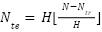
The number of retained test observations is then
| 
| (10) |
which ensures that every test forecast contains exactly observations. Any residual observations that cannot form a complete final horizon are excluded from the modeling dataset, exactly as implemented in the code.
A separate validation segment is taken from the end of the training period. Its length is defined as
| 
| (11) |
Thus, a 14-day validation period is used whenever sufficient historical training data remain; otherwise, the validation segment is reduced to seven days. The resulting chronological organization can be expressed as
| 
| (12) |
No random shuffling is introduced at the dataset level. Training windows are generated from the historical section with an internal step size of one observation, whereas the out-of-sample evaluation advances by one complete forecasting horizon. This distinction allows the model to exploit a dense set of training sequences while preserving non-overlapping daily forecast windows during final evaluation.
TimesNet Forecasting Architecture
The adopted model is a univariate TimesNet configured specifically for the TAS electricity-demand forecasting task. No static or historical exogenous variables are supplied. However, seven deterministic future-known calendar variables are provided to represent time-of-day, day-of-week, annual, and weekend effects. The historical electricity-demand sequence remains the principal forecasting input. The NeuralForecast implementation first maps the input sequence into a latent space, expands its temporal dimension from  to , processes the resulting representation through stacked TimesBlocks, and finally projects the latent features to the output space.
Let the standardized input batch be
| 
| (13) |
where  is the batch size, is the historical input length, and the final dimension equals one because only the electricity-demand series is modeled.
The input is mapped into a  -dimensional latent representation using a data embedding layer with positional information:
| 
| (14) |
where  denotes the positional representation and
 is the hidden dimension used in the present model. The positional embedding is activated in the implementation, while the dropout rate is set to 0.05.
Before entering the TimesBlocks, a linear transformation is applied along the temporal axis:
| 
| (15) |
Where
This operation extends the latent temporal representation from the historical length to the combined length
The procedure corresponds directly to the predict_linear layer in the NeuralForecast implementation.
The temporally aligned representation is then processed by  stacked TimesBlocks:
| 
| (16) |
where  denotes layer normalization. The adopted model uses
corresponding to two encoder layers. Each TimesBlock contains its own internal residual connection, while layer normalization is applied after the block output.
The final latent representation is projected back to the forecasting output space:
| 
| (17) |
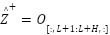
Only the final positions are retained as the forecast:
| 
| (18) |
After inverse scaling, the resulting output provides the demand forecast on the original measurement scale.
Both model training and validation use MAE:
| 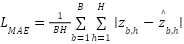
| (19) |
A balanced TimesNet configuration was adopted to increase representation capacity while maintaining manageable GPU-memory requirements. Each ensemble member uses a hidden dimension of 96, a convolutional hidden dimension of 128, seven dominant periods, six Inception kernels, two encoder layers, and a dropout rate of 0.05. MAE is used as both the training and validation loss. The maximum number of optimization steps is set to 5,000, with an initial learning rate of  and five scheduled reductions in the learning rate. Validation performance is evaluated every 100 training steps, and early stopping is activated after 10 consecutive validation checks without improvement. The training and validation batch sizes are both set to 8, while the training-window and inference-window batch sizes are set to 32 and 64, respectively. Standard temporal scaling is applied before model estimation. Three independently initialized models are trained using random seeds 42, 2024, and 3407, and their aligned forecasts are averaged to obtain the final TimesNet prediction. The complete experimental configuration is summarized in Table 1.
Multi-Periodicity Modeling with TimesBlock
The principal difference between TimesNet and conventional one-dimensional sequence models lies in the internal operation of TimesBlock. Instead of processing the latent sequence exclusively along the original time axis, each TimesBlock identifies several dominant periods and reorganizes the same temporal representation into multiple two-dimensional views. These views simultaneously expose variations within repeated periods and across successive periods.
Consider the input to a TimesBlock:  where
 . A real-valued fast Fourier transform is first applied along the temporal dimension:
| 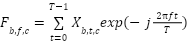
| (20) |
where  denotes the frequency index,
 denotes the latent channel, and
 .
A global frequency-amplitude representation is obtained by averaging the spectral magnitude across batches and latent channels:
| 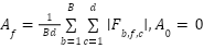
| (21) |
The experimental script does not apply an external tapering function before the TimesNet model; FFT-based period selection is performed internally on the temporally aligned latent representation. With an input length of  and a forecast horizon of
 , the combined temporal length is
 observations. At the 5-min sampling resolution, this sequence spans eight complete days, yielding a nominal discrete-frequency spacing of 1/8 = 0.125 cycles per day. The zero-frequency component is then excluded so that period selection focuses on oscillatory temporal behavior rather than the average sequence level.
The zero-frequency component is removed so that the period-selection mechanism focuses on temporal oscillations rather than the sequence's average level.
The  most influential frequencies are then selected:
| 
| (22) |
In the proposed forecasting framework,  meaning that five dominant periodic views are extracted in each TimesBlock. Importantly, these periods are not fixed manually as daily or weekly lags. They are adaptively derived from the latent representation via an FFT. The implementation computes the period using integer division, consistent with the actual NeuralForecast source code.
Because the combined sequence length,  , may not be exactly divisible by a detected period,
 , zero-padding is applied. The padded length is
| 
| (23) |
The padded one-dimensional sequence is then reorganized as a two-dimensional tensor:
| 
| (24) |
In this representation, one axis describes temporal positions within the selected period, whereas the other distinguishes successive occurrences of that period. Consequently, the model can examine both intra- and interperiod variation using standard two-dimensional convolutional operations. This is the central representation principle of TimesNet.
For each periodic view, a parameter-efficient Inception operation combines several receptive fields. Let denote the number of parallel kernels. The Inception transformation can be expressed as
| 
| (25) |
and the complete two-stage transformation is
| 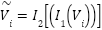
| (26) |
Because  in the adopted implementation, the parallel convolutional kernel sizes are
| 1×1,3×3,5×5,7×7,9×9,11×11 |
|
The first Inception block maps the 96-dimensional latent representation to 128 convolutional channels. Six parallel two-dimensional convolutional kernels provide different receptive fields, and the GELU activation function introduces nonlinear feature transformation. The second Inception block subsequently maps the extracted representation back to the 96-dimensional TimesNet hidden space. The outputs generated by the parallel kernels are averaged rather than concatenated.
After two-dimensional feature extraction, each representation is reshaped back to the original temporal organization and truncated to length . The period-specific features are then aggregated using normalized spectral amplitudes:
| 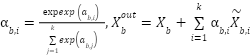
| (27) |
Where
| 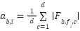
| (28) |
Thus, periodic components with stronger spectral evidence receive larger contributions to the current TimesBlock output. The final addition of the original input forms the residual connection.
The process is repeated in the second TimesBlock. Consequently, multi-periodicity is re-estimated from deeper representations rather than being detected only once from the raw load series. This allows the first block to extract an initial set of periodic features and the subsequent block to refine higher-level temporal structures. The complete mechanism is consistent with the TimesNet principle of adaptively representing multiple intraperiod and interperiod variations through structured two-dimensional tensors.
- Configuration of the adopted TimesNet forecasting model
Parameter | Setting |
Data resolution | 5 min |
Input size | 2,016 observations (7 days) |
Forecast horizon | 288 observations (1 day) |
Hidden size | 96 |
Convolutional hidden size | 128 |
Number of dominant periods | 7 |
Number of Inception kernels | 6 |
Encoder layers | 2 |
Dropout | 0.05 |
Training loss | MAE |
Validation loss | MAE |
Maximum training steps | 5,000 |
Initial learning rate | 3x10⁻⁴ |
Number of learning-rate decays | 5 |
Validation interval | 100 steps |
Early-stopping patience | 10 validation checks |
Training batch size | 8 |
Validation batch size | 8 |
Window batch size | 32 |
Inference-window batch size | 64 |
Internal training-window step size | 1 observation |
Temporal scaling | Standard |
Static exogenous variables | None |
Historical exogenous variables | None |
Future-known calendar variables | 7 |
Calendar variables | tod_sin, tod_cos, dow_sin, dow_cos, doy_sin, doy_cos, is_weekend |
Ensemble seeds | 42, 2024, 3407 |
Ensemble aggregation | Arithmetic mean |
Overall Algorithm and Forecasting Workflow
Figure 1 presents the complete TimesNet-based forecasting workflow adopted in this study, from the acquisition and preprocessing of the 2024 Tasmanian electricity demand series to rolling out-of-sample forecasting and comparative performance evaluation. The workflow preserves the chronological order of the observations and maintains a consistent 5-min, one-day-ahead forecasting configuration throughout model development and testing.
As illustrated in Figure 1, the forecasting procedure begins with the 2024 Tasmanian electricity demand series, in which the TOTALDEMAND variable is recorded at 5-min intervals. The raw timestamps and demand values are first converted into consistent datetime and numerical formats. Invalid records and duplicate timestamps are removed, and the remaining observations are chronologically sorted. A regular timestamp sequence is then constructed to verify temporal continuity and identify possible missing observations. This preprocessing stage ensures that all subsequent forecasting windows are generated from a clean, continuous, and correctly ordered time series.The processed dataset is subsequently divided according to temporal order. A total of 84,384 observations, corresponding to approximately 80.05% of the complete series, are assigned to model development, whereas the remaining 21,024 observations, or approximately 19.95%, are retained for final out-of-sample testing. The final 14 days of the model development period, comprising 4,032 observations, are reserved for validation. This chronological organization prevents future test observations from influencing model fitting, hyperparameter selection, early stopping, or validation-based model selection.
Supervised forecasting samples are then constructed from the univariate demand series. Each input sequence contains the previous seven complete days of electricity demand, equivalent to 2,016 observations at the 5-min resolution. The associated target comprises 288 observations, corresponding to a complete one-day-ahead forecasting horizon. This configuration provides sufficient historical context to represent repeated daily demand patterns, short-term variations, and relationships across consecutive days. In addition, seven deterministic future-known calendar encodings are supplied to TimesNet to represent time-of-day, day-of-week, annual, and weekend effects. At the same time, weather and other externally measured variables are excluded.
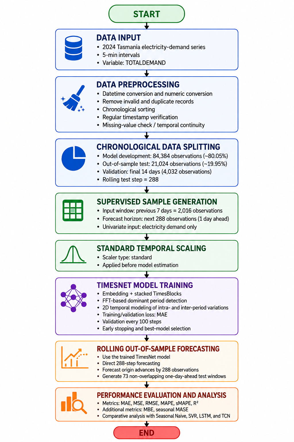
- Overall workflow of the TimesNet-based one-day-ahead electricity-load forecasting framework
Standard temporal scaling is applied before model estimation to improve numerical stability and facilitate model optimization. The scaled historical sequences are subsequently provided to TimesNet, where they are transformed into latent representations and processed through stacked TimesBlocks. Within each TimesBlock, the fast Fourier transform is used to identify dominant frequency components from the latent sequence. The corresponding periods are then used to reorganize the one-dimensional temporal representation into multiple two-dimensional tensors.
The two-dimensional representation enables TimesNet to model two complementary forms of temporal variation. The intraperiod dimension describes changes occurring within a repeated cycle, whereas the interperiod dimension represents differences among successive occurrences of that cycle. Two-dimensional convolutional operations extract features from these periodic views, and the period-specific outputs are adaptively combined according to their spectral importance. Consequently, TimesNet can represent several coexisting temporal structures rather than relying on a single fixed seasonal lag, recurrent state, or one-dimensional convolutional pathway.
The model is optimized using MAE as both the training and validation loss. Validation performance is examined every 100 optimization steps, while early stopping and best-model selection are used to reduce unnecessary training and limit overfitting. Only information from the model development and validation periods is used at this stage, and test observations are completely excluded from parameter estimation.
After training, the retained TimesNet model is applied through a rolling out-of-sample forecasting procedure. For each test origin, the model receives the most recent 2,016 historical observations and directly generates the following 288 demand values. The forecasting origin then advances by 288 observations, producing non-overlapping daily prediction windows. This process generates 73 complete one-day-ahead forecasts across the test period and ensures that each test observation is evaluated only once.
In the final stage, all out-of-sample predictions are concatenated in chronological order and compared with the corresponding observed demand values. Forecasting performance is assessed using MAE, MSE, RMSE, MAPE, sMAPE, and MBE, together with seasonal MASE, for evaluating systematic bias and scale-independent accuracy. The same test timestamps and metric definitions are used for TimesNet, Seasonal Naive, SVR, LSTM, and TCN. Therefore, the workflow provides a consistent basis for determining whether the explicit multi-periodicity representation of TimesNet offers a measurable forecasting advantage over the selected statistical, machine-learning, recurrent, and convolutional benchmarks.
EXPERIMENTAL SETUP
This section describes the dataset, data preparation, forecasting configuration, comparative models, evaluation criteria, and computational settings used in the experiments. The experimental design was developed to provide a consistent cross-paradigm comparison among statistical, machine-learning, deep-learning, and multi-periodicity-based forecasting methods. All models were evaluated on the same electricity-demand series and the same chronological test observations.
Dataset and Data Preparation
The experiments were conducted using the 2024 Tasmanian electricity demand dataset. The original data contain the timestamp variable SETTLEMENTDATE and the regional electricity-demand variable TOTALDEMAND. The forecasting problem uses a univariate electricity-demand target. Historical demand serves as the principal sequential input, while seven deterministic, future-known calendar encodings derived from the timestamps are supplied to TimesNet. No weather, socioeconomic, or other externally measured variables are included.
The timestamps were converted into a consistent datetime format, and the demand observations were converted into numerical values. Invalid records and duplicate timestamps were removed, and the remaining observations were then sorted chronologically. Following this cleaning procedure, the dataset contained 105,408 valid observations spanning from 1 January 2024 at 00:05 to 1 January 2025 at 00:00.
The sampling interval was determined from the modal difference between consecutive timestamps rather than being predefined manually. The detected interval was 5 min, corresponding to 288 observations per day and 2,016 observations per week. A complete regular timestamp grid was subsequently generated to identify possible discontinuities in the original series. The regularization procedure detected no missing observations before interpolation, corresponding to a missing-data rate of 0.00%. Consequently, although the preprocessing routine was configured to apply linear interpolation to internal gaps and forward or backward filling to unresolved boundary values, no demand observations required imputation. The final series was therefore continuous, regularly sampled, and free of missing target values.
The dataset was divided chronologically rather than randomly to preserve the temporal ordering of the forecasting problem and prevent information leakage. The split point was aligned with the complete one-day forecasting horizon of 288 observations. A total of 84,384 observations were assigned to model development, while 21,024 observations were retained for out-of-sample testing. These values correspond to actual proportions of approximately 80.05% and 19.95%, respectively. The training period ran from 1 January 2024 at 00:05 to 20 October 2024 at 00:00, while the test period ran from 20 October 2024 at 00:05 to 1 January 2025 at 00:00.
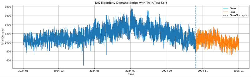
The test set contained 73 complete one-day forecasting windows, each comprising 288 observations. No residual observations were discarded because the complete series could be divided into horizon-aligned training and test sections. Figure 2 presents the complete Tasmanian electricity demand series, along with the chronological train–test division adopted in this study.
As shown in Figure 2, the model development period spans most of the annual demand series. It exhibits recurring daily behavior, short-duration fluctuations, gradual changes in demand levels, and several pronounced peaks and troughs. The seven-day input window therefore exposes the forecasting models to both high-resolution local variations and repeated temporal patterns across consecutive days.
The test period is strictly separated from model development and represents the final chronological portion of the dataset. It contains repeated intraday variations, rapid transitions, and local demand extremes, providing a meaningful out-of-sample evaluation of model performance. The vertical dashed line in Figure 2 identifies the boundary between the observations available for model development and those reserved exclusively for final testing. This chronological organization ensures that every test forecast is generated using only information available before the corresponding forecasting origin.
The final 14 days of the model-development period, comprising 4,032 observations, were reserved for validation. The remaining 80,352 observations were used for model fitting. The validation segment was used to monitor generalization performance, guide learning-rate adjustment, and apply early stopping, while the test data were not used during parameter estimation or model selection. The resulting chronological organization followed the sequence: Model fitting • Validation • Out-of-sample testing. This separation forms the basis of the common forecasting and benchmarking protocol described in the following subsection.
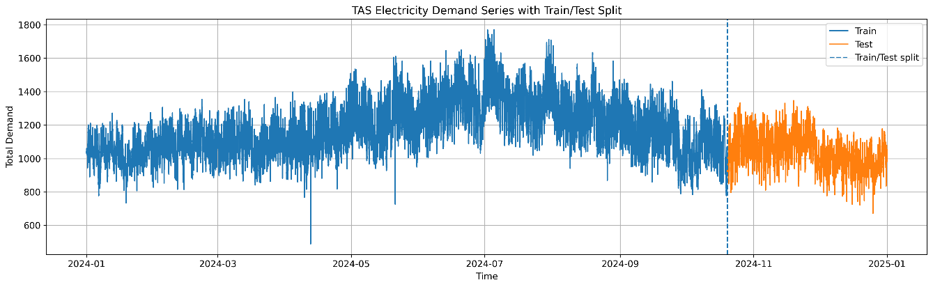
- Tasmania electricity-demand series and chronological train–test division
Forecasting Configuration and Fair Comparison Protocol
A common forecasting configuration was adopted to ensure that all evaluated methods were compared under equivalent external conditions. The detected sampling interval was 5 min, corresponding to 288 observations per day and 2,016 observations per week. The historical input length was therefore fixed at 2,016 observations, representing the previous seven complete days of electricity demand. In comparison, the forecast horizon was set to 288 observations, representing the complete following day. The forecasting task can be summarized as Previous 7 days (2,016 observations)→Following 1 day (288 observations).
The seven-day input window was selected for both temporal and methodological reasons. First, it contains seven complete daily cycles, enabling the models to learn recurring intraday demand behavior across different days of the week. Second, the window provides a complete weekly historical context for representing relationships across consecutive days. This sequential information is complemented by deterministic day-of-week and weekend encodings derived from the timestamps. Third, the relatively long, high-resolution sequence provides sufficient temporal information for TimesNet's FFT-based period-detection mechanism to identify several coexisting short- and long-period components. The 288-step horizon was selected because it corresponds to a complete operationally relevant day-ahead forecast rather than a sequence of isolated short-horizon predictions.
The chronological model-development set contained 84,384 observations, of which the final 4,032 observations, corresponding to 14 days, were reserved for validation. The out-of-sample test set contained 21,024 observations, forming 73 complete one-day forecasting windows. Training sequences were generated from the model development period, using densely overlapping historical windows where applicable. During final testing, the forecasting origin advanced by 288 observations after each prediction. This procedure generated non-overlapping one-day-ahead forecasts over the entire test period and prevented the same target observation from being evaluated more than once.
Comparison consistency was maintained at the target-series, chronological-partition, forecast-horizon, test-timestamp, and evaluation levels. All models were evaluated using the same cleaned Tasmania demand target, chronological test period, 288-step forecast horizon, forecast origins, observed target values, and metric definitions. The adopted TimesNet implementation additionally used deterministic future-known calendar encodings derived from the timestamps. These variables contained no future electricity-demand observations and were available at every forecasting origin. For models requiring a historical demand sequence, the available target history was restricted to the same seven-day period preceding each forecast origin. No future target observation beyond the corresponding forecasting origin was available during prediction.
The validation segment was used to monitor validation loss, guide the learning-rate schedule, and apply early stopping. The test set was not used during model fitting, validation monitoring, or training control. The fixed TimesNet configuration specified in Table 1 was retained throughout the complete out-of-sample evaluation. The resulting predictions were aligned to the same 21,024 test observations and evaluated using identical metric definitions.
The comparison protocol consisted of four stages. First, each method received the same chronologically cleaned target series. Second, each trainable model learned its own representation of the historical observations using only the model-development and validation periods. Third, all methods generated forecasts for the same sequence of 73 test windows. Finally, the predictions were concatenated chronologically and evaluated using the same observed values and performance criteria.
The purpose of this protocol was not to impose identical internal architectures or optimization algorithms on fundamentally different forecasting methods. Seasonal Naive, SVR, LSTM, TCN, and TimesNet use different learning principles and therefore require model-specific implementations. Instead, the protocol controls the target series, forecast horizon, chronological evaluation period, and metric definitions. Because the adopted TimesNet implementation additionally uses deterministic calendar encodings and ensemble averaging, the observed performance differences should be interpreted as differences between the complete forecasting implementations rather than as effects of architecture alone.
Comparative Models and Balanced TimesNet Implementation
Five forecasting methods were included in the comparative evaluation: Seasonal Naive, support vector regression (SVR), long short-term memory (LSTM), temporal convolutional network (TCN), and TimesNet. These methods were selected to provide a cross-paradigm benchmark spanning seasonal persistence, conventional nonlinear machine learning, recurrent sequence modeling, one-dimensional temporal convolution, and adaptive multi-period representation.
Seasonal Naive served as the statistical reference. It generates each future demand value using the corresponding observation from the previous seasonal cycle. Its inclusion determines how much forecasting information can be obtained directly from recurring historical behavior without parameter estimation or nonlinear representation learning. Because the Tasmania load series exhibits strong daily recurrence, Seasonal Naive provides a meaningful low-complexity benchmark for the complete 288-step day-ahead task.
SVR represented conventional machine learning. It learns a nonlinear mapping from historical demand data to future electricity load using kernel-based regression. Unlike deep learning models, SVR does not internally construct a hierarchy of temporal features. Its performance therefore indicates whether a conventional nonlinear mapping is sufficient to represent the high-resolution day-ahead forecasting relationship.
LSTM was included as the benchmark recurrent deep learning model. Its gated memory mechanism regulates the retention, updating, and transfer of historical information across the input sequence. This allows LSTM to model nonlinear dependencies over relatively long temporal intervals and provides an appropriate reference for evaluating whether explicit multi-period representation offers an advantage over recurrent temporal memory.
TCN represented convolution-based sequence learning. It uses causal and dilated one-dimensional convolutions to increase the temporal receptive field while preserving chronological direction. The comparison between TCN and TimesNet is particularly informative because both models use convolutional operations but organize temporal information differently. TCN processes the one-dimensional load sequence directly, whereas TimesNet first detects dominant periods and then reorganizes the sequence into multiple two-dimensional temporal views.
TimesNet was the principal model evaluated in this study. Within each TimesBlock, dominant frequency components are identified using a fast Fourier transform and converted into corresponding periods. The sequence is then reshaped for each selected period, so that intra- and interperiod variations can be processed simultaneously using two-dimensional convolutional operations. The period-specific representations are finally aggregated according to their spectral importance.
As summarized in Table 2, the comparison evaluates not only five individual models but also five distinct principles for representing electricity-demand behavior. Seasonal Naive assumes that the future resembles a previous seasonal cycle. SVR learns a nonlinear mapping from a predefined historical representation. LSTM transfers information through recurrent hidden states, while TCN extracts patterns using a fixed hierarchy of one-dimensional temporal filters. TimesNet differs in that it adaptively detects several dominant periods and jointly models changes within and across repeated cycles.
A balanced TimesNet configuration was adopted to increase model capacity while controlling GPU-memory consumption through relatively small batch and window sizes. Each ensemble member used a hidden dimension of 96, a convolutional hidden dimension of 128, seven dominant periods, six Inception kernels, two encoder layers, and a dropout rate of 0.05. MAE was used as both the training and validation loss. The maximum number of optimization steps was set to 5,000, with an initial learning rate of and five scheduled reductions in the learning rate. Validation performance was evaluated every 100 training steps, and early stopping was activated after 10 validation checks without improvement. The training and validation batch sizes were both 8, while the training-window and inference-window batch sizes were 32 and 64, respectively. Standard temporal scaling was applied. Seven deterministic future-known calendar variables were supplied, while static and historical exogenous variables were excluded. Three independently initialized models, seeded with 42, 2024, and 3407, were trained, and their aligned predictions were averaged to obtain the final TimesNet forecast.
The experimental program recorded the combined time required for model training, validation, and rolling out-of-sample prediction. Because these stages were timed jointly, the resulting value represents the total experimental runtime rather than isolated training time or per-window inference latency. From a computational perspective, the FFT-based period-detection stage has complexity O(TlogT), where  is the temporally aligned sequence length. The subsequent two-dimensional convolutional cost increases with the number of selected periods, the hidden dimensions, the kernel configurations, and the batch size. Processing seven periodic views with six parallel kernels introduces greater computational demand than the simpler benchmark implementations. In addition, using three independently trained ensemble members approximately triples the model-training workload compared with a single TimesNet run. Small training, validation, and window batch sizes were therefore adopted to control GPU-memory consumption.
For longer historical datasets with the same input and forecast lengths, the number of training windows increases approximately linearly with the number of available observations. At the same time, the memory required for a single batch is primarily determined by the fixed input length, forecast horizon, hidden dimensions, and batch size. This characteristic allows the framework to be extended to longer regional histories through mini-batch training. However, applications involving many regions, additional variables, or substantially longer input sequences would require additional memory management, distributed training, or adjustments to model capacity.
The benchmark was designed to evaluate TimesNet across fundamentally different forecasting paradigms rather than to provide an exhaustive ranking of all recently proposed Transformer architectures. Consequently, the reported results should be interpreted as evidence relative to Seasonal Naive, SVR, LSTM, and TCN under the adopted common protocol. No claim of superiority is made over untested architectures such as Informer, Autoformer, PatchTST, FEDformer, or iTransformer.
- Forecasting models used in the comparative evaluation
Category | Model | Main representation mechanism |
Statistical | Seasonal Naive | Direct seasonal recurrence |
Machine learning | SVR | Kernel-based nonlinear regression |
Deep learning | LSTM | Recurrent gated memory |
Deep learning | TCN | Causal and dilated one-dimensional temporal convolution |
Multi-period deep learning | TimesNet | Adaptive multi-period two-dimensional temporal modeling |
Evaluation Metrics
Forecasting performance was evaluated using five complementary measures: mean absolute error (MAE), mean squared error (MSE), root mean squared error (RMSE), mean absolute percentage error (MAPE), symmetric mean absolute percentage error (sMAPE), mean bias error (MBE), the coefficient of determination (), and seasonal mean absolute scaled error (seasonal MASE).
Let  and
 denote the observed and predicted demand values for the
 -th test observation, respectively, and let denote the total number of test predictions.
The MAE is defined as
| 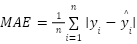
| (29) |
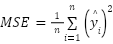
The MSE is calculated as
| 
| (30) |
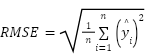
The RMSE is expressed as
| 
| (31) |
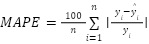
The MAPE measures the average absolute forecasting error relative to the observed demand:
| 
| (32) |
The coefficient of determination is defined as
| 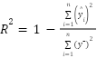
| (33) |
where  is the mean observed demand over the test period. Lower MAE, MSE, RMSE, and MAPE values indicate higher forecasting accuracy. In contrast, a laR-squared value indicates that the predicted series more effectively reproduces the variation in observed electricity demand.
Computational Environment and Reproducibility
The experiments were implemented in Python 3.12 using NeuralForecast 3.1.9 with a PyTorch 2.11.0+cu128 backend. Model training and forecasting were performed in Google Colab using a single CUDA-enabled GPU. The original execution log verified that GPU acceleration was available and used during both training and prediction. However, because Google Colab dynamically allocates computational hardware and the device name was not preserved in the original run, no unsupported claim regarding the exact GPU model or memory capacity is made. The reported execution time should therefore be interpreted in relation to the verified software configuration and the Google Colab GPU environment rather than as a hardware-independent benchmark.
The TimesNet configuration used to obtain the reported results employed a hidden dimension of 96, a convolutional hidden dimension of 128, seven dominant periods, six Inception kernels, two encoder layers, and a dropout rate of 0.05. The model was trained using MAE as both the training and validation loss. The maximum number of optimization steps was set to 5,000, the initial learning rate was 3×10⁻⁴, and five scheduled learning-rate reductions were employed. Validation performance was evaluated every 100 training steps, with an early-stopping patience of 10 validation checks. The training and validation batch sizes were both 8, while the training-window and inference-window batch sizes were 32 and 64, respectively. Standard temporal scaling was applied. Seven deterministic future-known calendar variables were supplied to the model, while static and historical exogenous variables were excluded.
The implementation automatically recorded the total time required for model fitting, validation, and rolling out-of-sample forecasting. Because these stages were timed jointly, the recorded value represents total execution time rather than separate training time or per-window inference latency. Separate measurements of parameter memory and model-specific inference latency were not recorded in the present implementation.
To reduce dependence on a single stochastic initialization, three TimesNet models were trained independently using random seeds 42, 2024, and 3407. For each ensemble member, the corresponding Python, NumPy, PyTorch, and CUDA random generators were initialized before model construction and training. The final TimesNet prediction was calculated as the arithmetic mean of the three aligned out-of-sample forecasts. Some GPU operations may remain nondeterministic across hardware and software environments; therefore, exact bitwise reproduction cannot be guaranteed.
The complete experimental configuration was stored together with the forecasting outputs. The saved information included the detected data frequency, input size, forecast horizon, train–test organization, validation length, target variable, model hyperparameters, deterministic calendar variables, ensemble seeds, package versions, GPU availability, and total execution time. The trained model, aligned out-of-sample predictions, performance tables, residual statistics, and generated figures were also retained. This procedure provides a transparent computational record and supports independent examination and reproduction of the reported forecasting results.
RESULTS AND DISCUSSION
Benchmark Accuracy and Comparative Improvement Analysis
The principal forecasting results of this study are presented in Table 3 and visualized in Figure 3. Table 3 provides the complete numerical comparison of the five evaluated models using MAE, MSE, RMSE, MAPE, and . In contrast, Figure 3 graphically illustrates the four most informative indicators, namely MAE, RMSE, MAPE, and . Since both presentations are based on the same test predictions, the table reports the exact quantitative results. At the same time, the figure highlights the relative rankings and performance gaps among the forecasting approaches. Together, they provide the central empirical evidence for assessing whether TimesNet's multi-periodicity modeling mechanism offers an advantage over statistical, machine-learning, recurrent, and convolutional forecasting methods.
- Forecasting Accuracy Comparison of TimesNet and Benchmark Models
Model | MAE | MSE | RMSE | MAPE |
|
TimesNet | 47.53 | 3625.65 | 60.21 | 4.66 | 0.6682 |
TCN | 87.43 | 10835.48 | 104.09 | 8.62 | 0.0085 |
SVR | 54.33 | 4766.55 | 69.04 | 5.40 | 0.5639 |
Seasonal Naive | 60.78 | 5994.83 | 77.43 | 5.95 | 0.4515 |
LSTM | 53.56 | 4697.58 | 68.54 | 5.32 | 0.5702 |
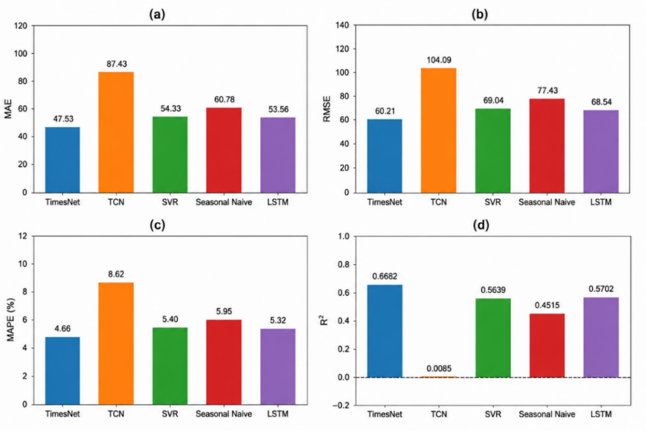
- Comparative forecasting performance of TimesNet and the benchmark models in terms of (a) MAE, (b) RMSE, (c) MAPE, and (d)
The results in Table 3 show that TimesNet achieves the best overall forecasting performance across all five evaluation metrics. It records the lowest MAE of 47.53, MSE of 3625.65, RMSE of 60.21, and MAPE of 4.66%, while simultaneously achieving the highest cap R squared of 0.6682. This consistent ranking is important because the superiority of TimesNet is not limited to a single error measure. The model performs best according to average absolute deviation, squared error, large-error sensitivity, relative percentage error, and goodness of fit. Therefore, the final ranking is not dependent on the choice of one particular metric.
Among the benchmark methods, LSTM provides the strongest overall performance, followed closely by SVR. LSTM achieves an MAE of 53.56, an RMSE of 68.54, a MAPE of 5.32%, and an of 0.5702, whereas SVR obtains corresponding values of 54.33, 69.04, 5.40%, and 0.5639. Although the difference between these two models is relatively small, both remain consistently behind TimesNet across all reported indicators.
Compared with LSTM, the strongest overall baseline, TimesNet reduces MAE by 11.26%, MSE by 22.82%, RMSE by 12.15%, and MAPE by 12.41%. At the same time, its increases from 0.5702 to 0.6682, an absolute improvement of 0.0980. This difference is particularly notable because LSTM already provides a strong nonlinear recurrent representation of the historical load sequence. The additional improvement achieved by TimesNet indicates that explicit multi-period temporal modeling provides useful information beyond conventional recurrent memory.
A similar pattern is observed relative to SVR. TimesNet reduces MAE by 12.52%, MSE by 23.94%, RMSE by 12.79%, and MAPE by 13.70%, while increasing by 0.1043. These differences show that kernel-based nonlinear regression can capture a substantial part of the load dynamics, but its fixed input–output mapping remains less effective than the multi-period representation learned by TimesNet.
The advantage over Seasonal Naive is more pronounced. TimesNet reduces MAE by 21.80%, MSE by 39.52%, RMSE by 22.24%, and MAPE by 21.68%. The value also rises from 0.4515 to 0.6682. This comparison is especially relevant because Seasonal Naive directly exploits recurring load behavior. Its reasonable performance confirms that the Tasmania electricity-demand series contains substantial seasonal regularity. However, TimesNet clearly performs better, suggesting that direct seasonal repetition alone cannot fully represent the nonlinear changes and variations occurring within and across repeated demand cycles.
TCN produces the weakest results in the present experimental setting, with an MAE of 87.43, RMSE of 104.09, MAPE of 8.62%, and of only 0.0085. Relative to TCN, TimesNet reduces MAE by 45.64%, MSE by 66.54%, RMSE by 42.16%, and MAPE by 45.94%. The very low of TCN indicates that its predictions reproduce only a limited proportion of the observed load variation. Although both TCN and TimesNet use convolutional operations, their markedly different performance suggests that the way temporal information is organized is critical. TCN applies convolution directly along the one-dimensional temporal sequence, whereas TimesNet first restructures the sequence according to several dominant periodicities and then models intraperiod and interperiod variation in two dimensions.
Figure 3 reinforces the numerical findings reported in Table 3. In Figure 3(a) to Figure 3(c), TimesNet consistently has the shortest bars for MAE, RMSE, and MAPE, indicating the lowest forecasting errors. In contrast, Figure 3(d) shows that TimesNet has the highest , demonstrating the strongest agreement between the predicted and observed demand variations. The visual separation is particularly evident relative to TCN and Seasonal Naive, while TimesNet also maintains a clear advantage over the stronger LSTM and SVR baselines.
The combined evidence from Table 3 and Figure 3 therefore constitutes the principal result of this study. Across statistical, machine-learning, recurrent deep-learning, and convolution-based forecasting paradigms, TimesNet provides the most accurate overall predictions for the TAS 2024 electricity-demand series. The improvement is consistent across all five metrics and is especially meaningful when compared with LSTM, which represents the strongest baseline in the benchmark.
These findings are consistent with the usefulness of explicit multi-period temporal representation for short-term load forecasting. TimesNet identifies several dominant periodic structures and jointly represents variations within and across repeated cycles. However, because the adopted TimesNet implementation also incorporates deterministic calendar encodings and three-member ensemble averaging, the present comparison does not isolate the independent contribution of the multi-periodicity mechanism. The results should therefore be interpreted as the performance of the complete adopted TimesNet implementation under the common evaluation protocol.
Overall, Table 3 and Figure 3 provide the final quantitative answer to the main research question of this study. Under the common forecasting protocol, TimesNet achieves the lowest prediction errors and the highest goodness of fit among all evaluated models. These results establish TimesNet as the best-performing forecasting method in the present experiment and provide the central empirical foundation for the subsequent analyses of error behavior, temporal profile tracking, and forecast-horizon robustness.
Error Distribution, Bias, and Forecast Robustness
While the aggregate metrics presented in the previous section show that TimesNet obtained the lowest overall errors under the adopted experimental setting over the benchmark models, average performance measures alone do not fully reveal how forecasting errors are distributed across individual test samples. Two models with similar average errors may exhibit substantially different levels of dispersion, extreme deviations, and sensitivity to difficult forecasting periods. Therefore, a distributional analysis is required to further examine the consistency and robustness of the competing models. Figure 4 presents the distributions of the absolute percentage error (APE) for TimesNet, LSTM, Seasonal Naive, SVR, and TCN.

- Distribution of absolute percentage errors for TimesNet and the benchmark forecasting models
As shown in Figure 4, the error distributions provide further evidence supporting the comparative results reported in the previous section. TimesNet exhibits the most favorable overall distribution, with the largest proportion of observations concentrated in the low-APE region. Its frequency decreases rapidly as the error magnitude increases, while relatively few observations occur in the high-error tail. This pattern indicates that the superior MAPE, MAE, and RMSE values obtained by TimesNet are not due to a limited number of highly accurate predictions; rather, they reflect consistently small forecasting errors across a large portion of the test set. The comparatively short and sparse right tail also suggests greater robustness against large pointwise deviations.
LSTM and SVR display broadly similar right-skewed distributions, with most predictions also concentrated at relatively low APE values. However, their distributions extend farther into the moderate- and high-error regions than that of TimesNet. This observation is consistent with their previously reported slightly higher aggregate errors. Although both models can provide accurate predictions for a considerable number of observations, the greater frequency of moderate errors and the longer right tails indicate less stable forecasting performance than TimesNet.
The Seasonal Naive model exhibits a broader error distribution and a more pronounced right tail. Compared with learning-based models, a larger proportion of its forecasts fall within the intermediate-error range, and isolated errors extend beyond approximately 30%. This broader dispersion indicates that simply repeating historical seasonal patterns cannot adequately capture all short-term changes in electricity demand. Consequently, the model is more vulnerable when the current load behavior deviates from previously observed seasonal patterns.
The clearest contrast is observed for TCN. Unlike the other models, its error distribution is not strongly concentrated near zero but instead peaks at a noticeably higher APE range. The distribution remains broad and extends beyond 40%, indicating both a higher typical forecasting error and a substantially greater occurrence of large deviations. This behavior explains the markedly poorer MAE, RMSE, and MAPE values and the near-zero reported in the preceding analysis. Therefore, the weak aggregate performance of TCN is not due solely to a small number of extreme outliers; it reflects a broader, less favorable error distribution across the test set.
Overall, Figure 4 complements the aggregate metric comparison by showing that TimesNet achieves not only the lowest average forecasting error but also the most concentrated and stable error distribution. Its strong concentration in the low-APE region and limited high-error tail demonstrate better forecasting consistency and robustness than the benchmark models. These findings provide distribution-level evidence that TimesNet's performance advantage is maintained across individual forecasting instances, rather than being driven solely by average statistics.
Load Profile Tracking and Temporal Forecast Characteristics
The distributional analysis in Section 5.2 showed that TimesNet produces a greater concentration of low-error predictions and a more limited high-error tail than the benchmark models. However, error distributions do not indicate when forecasting deviations occur or whether a model can accurately reproduce the temporal evolution of electricity demand. To complement the aggregate and distribution-level analyses, Figure 5 compares the actual and forecasted load profiles over the first seven days of the test period. This comparison provides a direct assessment of each model’s ability to preserve daily load cycles, follow rapid transitions, and reproduce the timing and magnitude of peaks and troughs.
As shown in Figure 5, all models capture the general existence of recurring daily demand patterns. Still, substantial differences are observed in temporal alignment, amplitude representation, and responsiveness to short-term load variations. These differences provide a time-domain explanation for the comparative error statistics and APE distributions discussed in the preceding sections.
The Seasonal Naive model reproduces the broad daily periodicity of the load series because its forecasts are directly based on previously observed seasonal behavior. Nevertheless, the predicted profiles frequently differ from the actual demand in both amplitude and local trajectory. Several peaks and troughs are either overestimated or underestimated, particularly when the load pattern changes from one day to the next. This behavior indicates that the model can preserve repetitive temporal structure but has limited ability to adapt to changes in the magnitude and shape of the current load profile. Consequently, the accumulated deviations across the seven days are consistent with its broader APE distribution and higher overall forecasting errors.
SVR provides substantially better temporal tracking than the Seasonal Naive benchmark. Its forecasts generally follow the major rising and falling trends and reproduce the timing of many daily peaks and valleys. However, noticeable discrepancies persist during periods of rapid change or unusually high demand. In several cases, the predicted curve departs from the actual series near extreme peaks and sharp transitions. This suggests that SVR captures the dominant nonlinear relationship in the data but may still smooth or distort some short-term variations. These localized mismatches explain why SVR achieves relatively strong overall performance while remaining inferior to TimesNet in the aggregate metrics.
LSTM also captures the recurring daily cycle and follows the general direction of load evolution. Compared with the actual series, however, its predictions are visibly smoother, and the amplitudes of several sharp peaks and deep troughs are reduced. This smoothing effect is particularly evident during abrupt changes in demand, where the forecast curve responds more gradually than the actual load. As a result, LSTM performs well during regular periods but may lose accuracy when the demand profile changes rapidly. This temporal behavior is consistent with the moderate right tail observed in its APE distribution.
The weakest temporal tracking behavior is observed for TCN. Although the model reproduces the approximate periodic structure of the demand series, its forecast amplitude is considerably compressed during several portions of the seven days. The discrepancy becomes especially pronounced during high-load intervals, where TCN repeatedly underestimates the actual demand and fails to reproduce the magnitude of major peaks. In addition, the predicted profile shows limited adaptation to changes in the daily load level. These systematic temporal deviations confirm that the poor performance of TCN is not attributable only to isolated forecasting errors. Instead, they reflect persistent difficulty in representing the evolving magnitude and short-term dynamics of the demand series, which is consistent with its high MAE, RMSE, and MAPE and near-zero .
TimesNet provides the closest overall correspondence between the predicted and actual load profiles. The forecast curve generally follows both the direction and timing of the observed demand, including repeated daily cycles, rising and falling transitions, and changes in load magnitude across successive days. Compared with the benchmark models, TimesNet more accurately preserves the shape of the actual profile and exhibits smaller deviations around most peaks and troughs. Some discrepancies remain during the most extreme demand variations, particularly near several sharp peaks, but these deviations are less persistent than those observed for the competing models.
An important characteristic of the TimesNet forecast is its ability to adapt to changes in the daily load level rather than merely reproducing an average or previously observed profile. The model follows not only the recurring periodic behavior but also the variation in peak heights, valley depths, and intra-day transitions across the seven days. This improved amplitude fidelity and temporal responsiveness help explain why TimesNet simultaneously achieves the lowest MAE, RMSE, and MAPE and the highest . The visual results, therefore, reinforce the findings from the previous sections by showing that the model’s superior numerical performance is directly associated with more accurate temporal tracking.
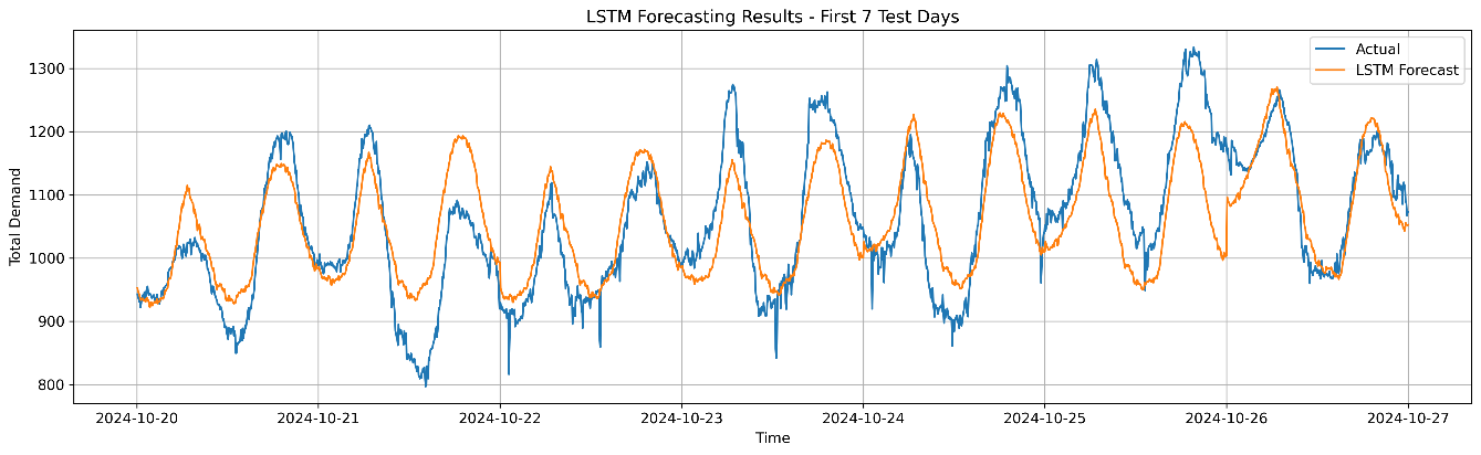
|
(a) LSTM |
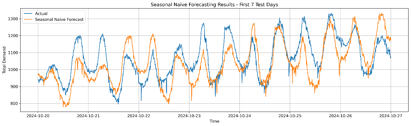
|
(b) Seasonal Naive |
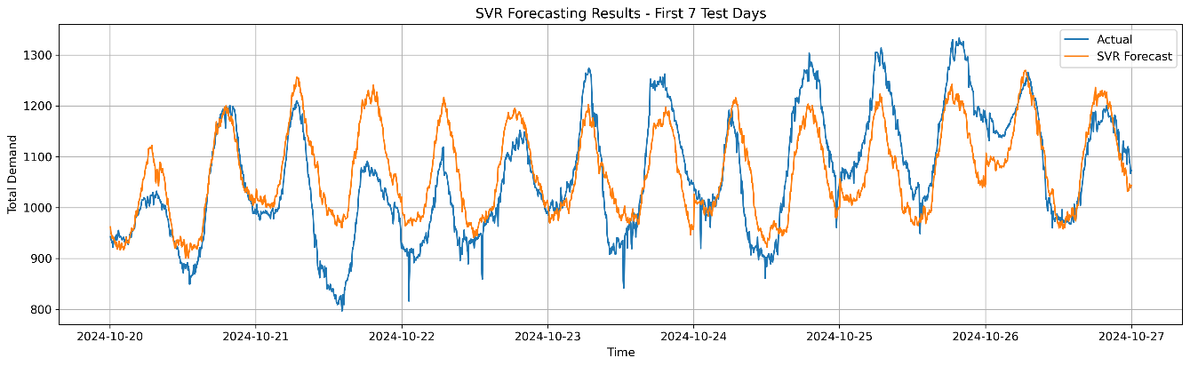
|
(c) SVR |
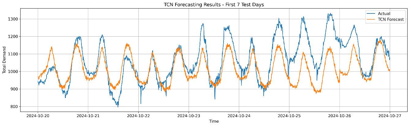
|
(d) TCN |
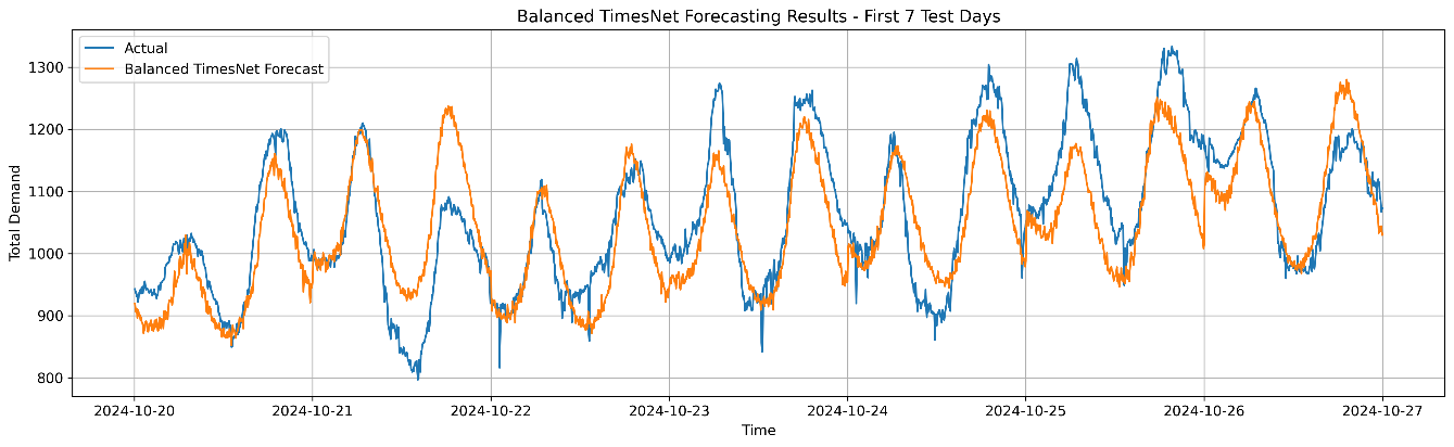
|
(e) TimesNet |
- Seven-day load-profile tracking performance of (a) LSTM, (b) Seasonal Naive, (c) SVR, (d) TCN, and (e) TimesNet
Overall, Figure 5 demonstrates that forecasting performance depends not only on identifying the recurring daily cycle but also on reproducing changing amplitudes and short-term transitions. Seasonal Naive retains basic periodicity but lacks adaptability, SVR and LSTM provide stronger profile tracking with remaining local deviations, and TCN exhibits pronounced amplitude underestimation. In contrast, TimesNet achieves the most balanced performance across temporal alignment, profile-shape preservation, and adaptation to changing demand levels. Together with the aggregate metrics and error-distribution results, this time-domain analysis provides further evidence of TimesNet's greater consistency and robustness in short-term load forecasting.
Forecast Robustness Across the One-Day-Ahead Horizon
The preceding analysis showed that TimesNet achieves the best aggregate forecasting accuracy, a favorable distribution of pointwise errors, and strong temporal tracking of the actual load profile. However, these results do not reveal whether the forecasting advantage is maintained consistently throughout the day-ahead prediction window. In multi-step forecasting, prediction difficulty may vary considerably with the forecast position because different horizon steps correspond to different load regimes, transition periods, peaks, and valleys. Therefore, Figure 6 examines the variation in MAPE across the complete one-day-ahead forecasting horizon for TimesNet and the benchmark models.
As shown in Figure 6, the horizon-wise error patterns are clearly non-uniform for all models. MAPE does not increase continuously with the forecast step; instead, it rises and falls across different portions of the prediction window. This behavior indicates that forecasting difficulty is influenced not only by increasing forecast horizon length but also by the temporal characteristics of the load profile at each horizon position. Periods containing rapid demand transitions and pronounced variations tend to produce larger errors, whereas more stable portions of the daily cycle are generally predicted more accurately.
TimesNet exhibits the most favorable overall horizon-wise error profile. Its MAPE remains relatively low during the early forecast steps, increases gradually through the middle portion of the horizon, and then decreases again toward the later steps. Although a local maximum is observed around the middle of the forecasting window, the error remains below that of the weakest benchmark and declines substantially in the final portion of the horizon. More importantly, the curve varies comparatively smoothly, indicating that the model maintains stable predictive behavior across successive forecast positions rather than exhibiting frequent abrupt deterioration.
The TimesNet error pattern also reveals that its forecasting advantage is not restricted to only the first few prediction steps. The model remains competitive throughout the entire forecast window, including the more difficult middle-horizon region. This finding is particularly important for day-ahead load forecasting, where a model must generate all future values simultaneously, and reliable performance is required across the entire prediction horizon. The comparatively low and smooth horizon-wise MAPE therefore provides further evidence of the model’s robustness in multi-step forecasting.
LSTM also achieves relatively low errors at the beginning of the forecast horizon. However, its MAPE increases substantially as the horizon lengthens and remains elevated for much of the middle section. The curve subsequently declines toward the final forecast steps. This pattern suggests that LSTM can provide accurate predictions for some temporal regions but experiences greater difficulty in the middle portion of the daily forecast window. The higher error level over an extended range of horizon steps is consistent with the smoothing behavior observed in Figure 5, where several peaks and rapid transitions were not fully reproduced.
SVR displays a broadly similar horizon-dependent pattern. The error begins at a relatively low level, increases sharply toward the first major high-error region, and remains comparatively elevated throughout much of the middle horizon before declining in the later steps. Several local fluctuations are also visible, indicating variable sensitivity to different temporal positions. Although SVR maintains reasonable performance overall, its horizon-wise error is generally higher than that of TimesNet across important portions of the prediction window. This result is consistent with the localized profile mismatches observed in the seven-day tracking analysis.
The Seasonal Naive model exhibits higher errors at the beginning of the horizon and a broader high-error region around the middle forecast steps. Its MAPE reaches its largest values in approximately the same general portion of the horizon where several learning-based models also experience increased difficulty. However, the magnitude of the error is greater, reflecting the model’s limited ability to adjust when the future load pattern differs from the historical seasonal reference. The subsequent decrease in MAPE toward the later horizon indicates that the model performs better when the corresponding load regime is more compatible with its repeated seasonal pattern.
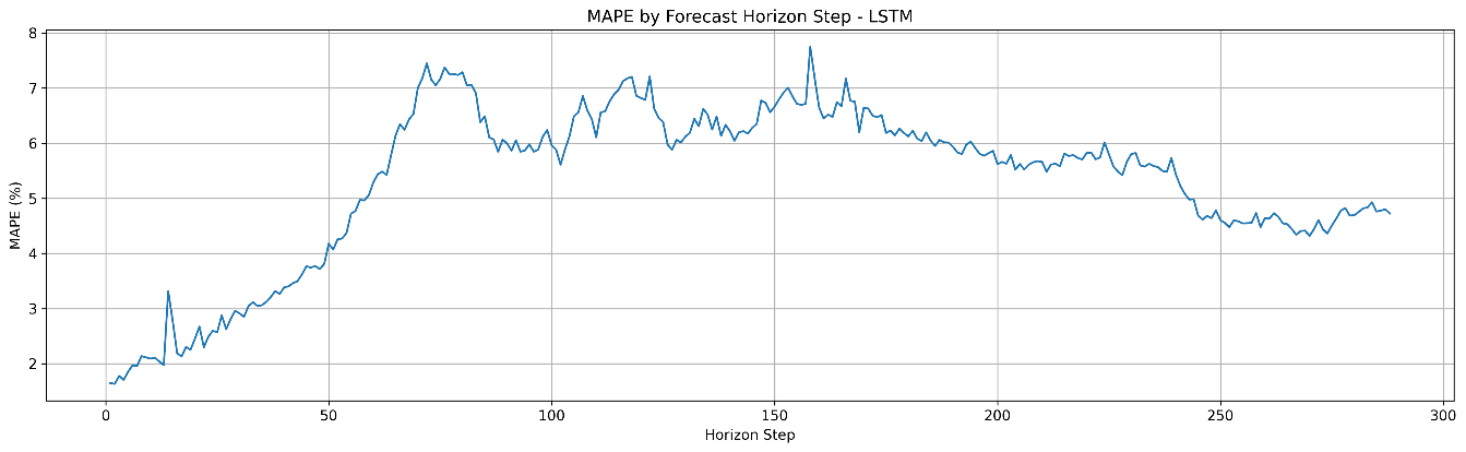
|
(a) LSTM |
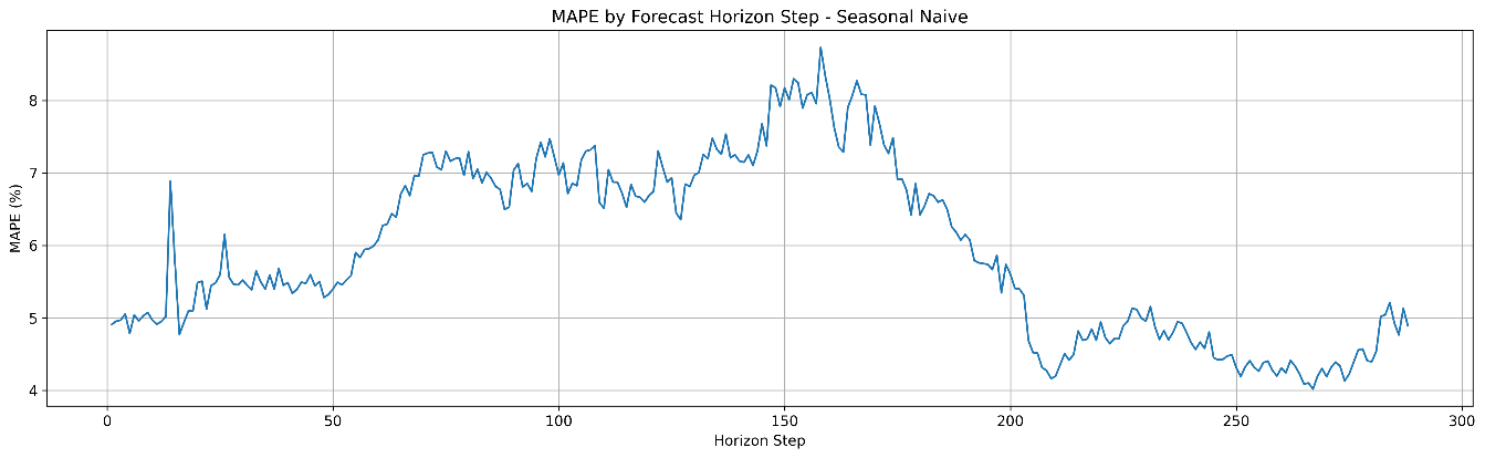
|
(b) Seasonal Naive |
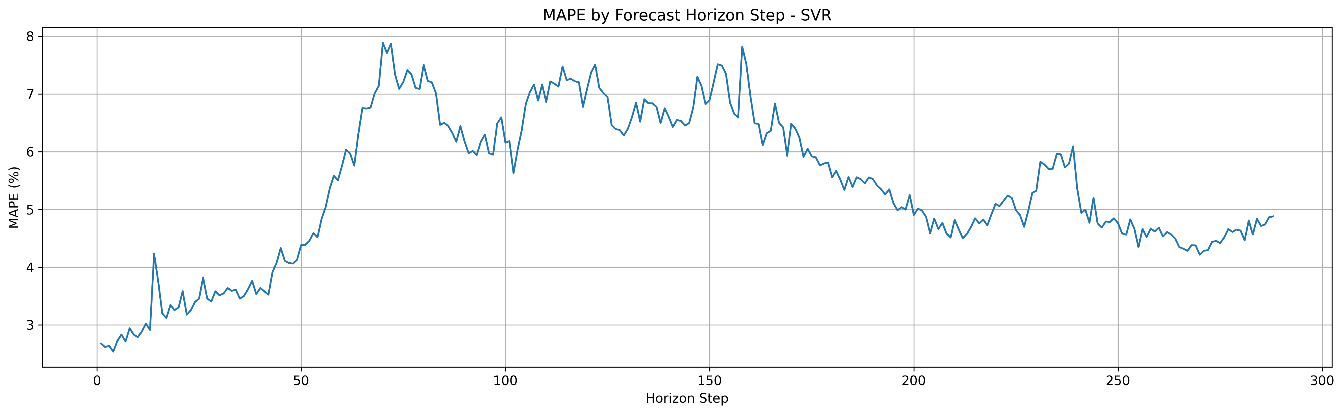
|
(c) SVR |
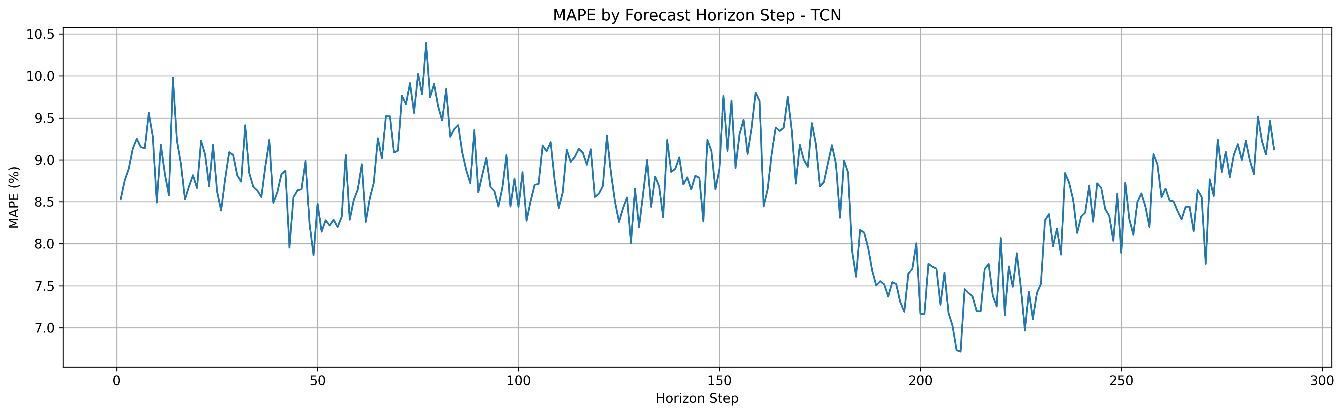
|
(d) TCN |
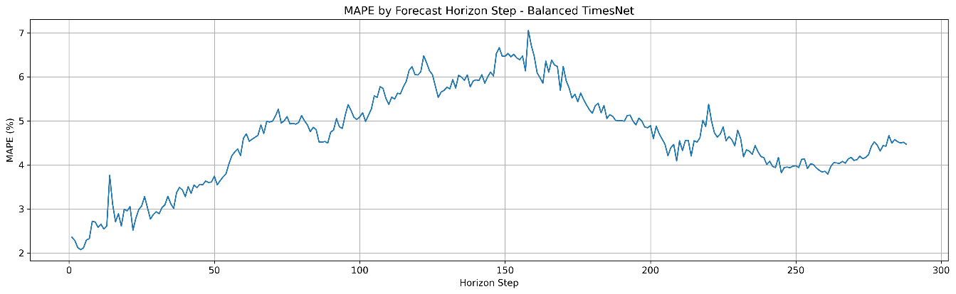
|
(e) TimesNet |
- MAPE variation across the 288-step one-day-ahead forecasting horizon for (a) LSTM, (b) Seasonal Naive, (c) SVR, (d) TCN, and (e) TimesNet
TCN presents the least favorable horizon-wise behavior. Its MAPE remains consistently high throughout most of the forecasting horizon, with repeated fluctuations and several pronounced peaks. Unlike the other models, TCN does not benefit from a sustained low-error region at the beginning of the horizon, and its performance remains comparatively weak even during later forecast steps. The persistent error level indicates that a narrow subset of difficult horizon positions does not cause its poor aggregate results. Instead, the model experiences systematic difficulty forecasting across much of the day-ahead sequence.
A particularly important observation from Figure 6 is that the errors of most models are highest around the middle region of the forecast horizon rather than at the final forecast step. Therefore, the results do not support a simple assumption that forecasting error increases monotonically with prediction distance. Instead, the variation appears strongly associated with changes in the temporal characteristics of electricity demand. Horizon positions corresponding to more complex load transitions are more difficult to predict, whereas relatively stable periods yield lower forecasting errors. This interpretation is also consistent with the seven-day load-profile analysis in Figure 5, where the largest deviations tended to occur around pronounced peaks, troughs, and rapid changes in demand.
Overall, Figure 6 extends the previous analyses by demonstrating that TimesNet maintains comparatively stable forecasting accuracy across the complete one-day-ahead horizon. While all models exhibit horizon-dependent error variation, TimesNet achieves a more favorable balance among low overall MAPE, smoother error variation, and reduced sensitivity to difficult forecast positions. Together with the aggregate metrics, APE distributions, and temporal tracking results, the horizon-wise analysis indicates that the observed advantage of TimesNet is not confined to a specific evaluation measure or a limited portion of the test sequence, but is maintained across multiple dimensions of forecasting performance.
Multi-Periodicity Interpretation and Computational Trade-Offs
The results presented in Section 5.1 to Section 5.4 provide a consistent view of TimesNet's forecasting behavior from several complementary perspectives. The model achieves the best aggregate accuracy, exhibits a stronger concentration of low pointwise errors, follows the observed load trajectory more closely, and maintains comparatively stable performance across the complete one-day-ahead forecasting horizon. Taken together, these findings suggest that the performance advantage of TimesNet is associated not only with lower average error but also with a more effective representation of the recurring and time-varying structures embedded in the electricity-demand series.
Electricity demand is inherently characterized by temporal patterns operating at different scales. At the 5-min resolution considered in this study, the load series contains short-term fluctuations within individual hours, recurring intra-day transitions, and the broader daily cycle represented by the 288-step forecasting horizon. These patterns do not contribute equally throughout the day. Stable periods, rapid ramps, peaks, and valleys introduce different forecasting difficulties, as demonstrated by the horizon-dependent MAPE variations in Figure 6. Consequently, an effective forecasting model must represent more than a single dominant periodic pattern; it must also accommodate interactions among different temporal structures and changing load regimes.
The empirical behavior of TimesNet is consistent with this requirement. In the seven-day tracking analysis, the model reproduced both the broad daily demand pattern and many of the shorter-term variations occurring within each daily cycle. Unlike the Seasonal Naive model, which primarily preserves historical periodicity, TimesNet showed greater adaptability when the amplitude and shape of the load profile varied across successive days. Similarly, compared with LSTM and SVR, it generally maintained better agreement with the actual demand during transitions between low- and high-load periods. These observations suggest that the model is better able to combine recurring temporal information with evolving local demand characteristics.
The horizon-wise analysis provides further support for this interpretation. The forecasting error did not increase monotonically with the prediction step; instead, it varied across different portions of the daily cycle. TimesNet maintained relatively favorable performance across these changing temporal regions, including the more difficult middle portion of the forecast horizon. This behavior indicates that its forecasting capability is not confined to a particular time position or a single repetitive structure. Rather, the model appears to provide a more balanced representation of the different temporal patterns encountered throughout the complete day-ahead sequence.
The error-distribution results lead to a similar conclusion. TimesNet produced a high concentration of observations in the low-APE region and comparatively fewer large deviations. This suggests that the model’s advantage is not driven only by accurate predictions during regular or easily predictable periods. Instead, the improvement is observed across a broader range of forecasting conditions. When considered together with the temporal tracking and horizon-wise results, the reduced error dispersion is consistent with a model that can represent both repeated load patterns and variations around those patterns more effectively.
These improvements, however, should be considered together with computational complexity. Simple methods such as Seasonal Naive have minimal training requirements and remain attractive when simplicity of implementation and computational cost are the main priorities. SVR also achieves competitive forecasting accuracy within a relatively conventional modeling framework, although its computational requirements may depend on the training set size and kernel configuration. LSTM and TCN introduce deeper temporal representation capabilities but require iterative training and model-specific configuration.
TimesNet involves a more sophisticated deep-learning architecture and therefore introduces additional computational overhead compared with simple statistical and conventional machine-learning benchmarks. Its practical advantage should consequently be evaluated as an accuracy–complexity trade-off rather than solely in terms of predictive performance. In applications where forecasting errors directly affect scheduling, reserve allocation, energy procurement, or other operational decisions, the improved accuracy and greater robustness may justify the additional computational effort. In contrast, simpler models may remain suitable for resource-constrained applications in which moderate forecasting accuracy is acceptable.
Importantly, the present results indicate that improvements across several independent evaluation dimensions accompany the additional model complexity. TimesNet not only achieves a lower average MAPE but also delivers better overall error metrics, a more favorable APE distribution, stronger load-profile tracking, and more stable horizon-wise performance. Therefore, the computational cost is associated with a broader improvement in forecasting quality rather than an isolated gain in a single metric.
Overall, the findings suggest that the main strength of TimesNet lies in its ability to capture the multi-periodic, non-uniform temporal characteristics of electricity demand within a unified forecasting framework. Its improved treatment of recurring daily structure, local variations, and horizon-dependent forecasting difficulty provides a plausible explanation for the consistent performance gains observed throughout this study. Although this capability requires greater computational complexity than simpler benchmarks, the resulting improvements in accuracy, consistency, and robustness indicate a favorable trade-off for applications that prioritize reliable one-day-ahead load forecasting.
CONCLUSION
This study evaluated TimesNet for one-day-ahead short-term load forecasting using the 2024 Tasmanian electricity demand series at a 5-min temporal resolution. The forecasting problem was formulated as a direct 288-step task, in which the previous seven days, corresponding to 2,016 observations, were used to predict the next day. The adopted TimesNet implementation combined explicit multi-periodicity modeling with seven deterministic future-known calendar encodings and three-member ensemble averaging. Its performance was compared with Seasonal Naive, support vector regression, long short-term memory, and temporal convolutional network models using the same target series, chronological test period, forecast horizon, test observations, and evaluation definitions.
Under the adopted experimental conditions, TimesNet achieved the best observed overall performance among the five evaluated methods, with an MAE of 47.53, an RMSE of 60.21, a MAPE of 4.66%, an sMAPE of 4.63%, and an of 0.6682. Compared with LSTM, the strongest overall benchmark, TimesNet reduced MAE, RMSE, and MAPE by 11.26%, 12.15%, and 12.41%, respectively. Its MBE of 1.28 indicates limited systematic bias, while its seasonal MASE of 0.726 demonstrates performance superior to the daily seasonal reference. The observed advantage was therefore consistent across absolute-error, percentage-error, goodness-of-fit, bias, and scale-independent measures.
The distributional, temporal, and horizon-wise analyses provided additional insight into the forecasting behavior of the evaluated models. TimesNet produced a greater concentration of predictions in the low-error region and comparatively fewer large pointwise deviations. It also more closely followed the observed seven-day load profile, particularly during changes in demand amplitude and transitions between low- and high-load periods. Over the full 288-step prediction horizon, its forecasting errors remained relatively stable. Forecasting difficulty varied according to the temporal position within the daily load cycle rather than increasing monotonically with forecast distance.
The main scientific contribution of this study is a controlled cross-paradigm evaluation of a TimesNet-based forecasting implementation for high-resolution day-ahead electricity-demand prediction. The findings are consistent with the usefulness of reorganizing a one-dimensional temporal sequence into several period-dependent two-dimensional representations that jointly describe intraperiod and interperiod variation. However, the adopted implementation also uses deterministic calendar encodings and three-member ensemble averaging. Consequently, the reported improvement represents the performance of the complete TimesNet implementation and should not be attributed exclusively to the multi-periodicity mechanism without further ablation experiments.
From a practical perspective, more accurate and temporally stable day-ahead forecasts can support generation scheduling, reserve allocation, electricity procurement, demand-response planning, and other operational decisions in modern power systems. Nevertheless, TimesNet requires greater architectural and training complexity than simple approaches such as Seasonal Naive. The present implementation recorded the combined model training and rolling prediction time, but separate inference latency, memory consumption, energy use, and computational cost were not consistently measured for every benchmark model. Its practical application should therefore be considered as an accuracy–complexity trade-off, particularly in resource-constrained or real-time environments.
Several limitations should be acknowledged. First, the experiments used a single electricity-demand target from a single region and calendar year; therefore, the findings should not be interpreted as evidence of universal superiority across electricity markets, seasons, or sampling resolutions. Second, although deterministic time-of-day, day-of-week, annual, and weekend encodings were included, weather conditions, public holidays, special events, and socioeconomic variables were not considered. This limitation may reduce forecasting accuracy during abnormal or externally driven demand conditions. Third, the benchmark did not include additional recent Transformer-based models such as Informer, Autoformer, FEDformer, PatchTST, or iTransformer. Fourth, TimesNet was implemented using a fixed, balanced configuration rather than an exhaustive hyperparameter optimization procedure, and the adopted setting may therefore not represent its maximum attainable performance. Fifth, the final TimesNet forecast was obtained by averaging three models initialized with fixed random seeds. In contrast, the complete benchmark was not repeated across multiple independent seed sets for every neural model. Confidence intervals and formal statistical significance tests were also not included. The reported performance differences should consequently be interpreted as empirical improvements under the adopted experimental setting rather than as definitive statistical evidence of superiority. Finally, because the benchmark models did not necessarily receive the same auxiliary calendar inputs or use the same ensemble strategy, the comparison is limited to the target series and evaluation protocol. Still, it does not isolate the effect of architecture alone.
Future work should evaluate TimesNet across multiple regions, years, seasons, and forecasting resolutions using repeated rolling-origin experiments. Paired statistical procedures, such as the Diebold–Mariano test or the Wilcoxon signed-rank test, should be combined with confidence intervals to determine whether the observed improvements remain statistically significant. Comparisons with recent Transformer-based forecasting architectures should also be conducted under equivalent input information, tuning budgets, and evaluation conditions. Systematic hyperparameter optimization, sensitivity analysis, and ablation experiments are required to quantify the individual contributions of dominant-period selection, hidden dimensions, encoder depth, Inception kernels, deterministic calendar encodings, and ensemble averaging. Further extensions should incorporate weather variables, public holiday indicators, special event information, and socioeconomic factors, particularly during periods of extreme demand and abnormal operating conditions. Additional promising directions include probabilistic forecasting, calibrated prediction intervals, transfer learning across regions, online adaptation to concept drift, and deployment-oriented evaluation of inference latency, energy consumption, memory requirements, and real-time scalability.
REFERENCES
- S. Akhtar, S. Shahzad, A. Zaheer, H. S. Ullah, H. Kilic, R. Gono, M. Jasiński, and Z. Leonowicz, “Short-term load forecasting models: A review of challenges, progress, and the road ahead,” Energies, vol. 16, no. 10, p. 4060, 2023, https://doi.org/10.3390/en16104060.
- M. G. Pinheiro, S. C. Madeira, and A. P. Francisco, “Short-term electricity load forecasting—A systematic approach from system level to secondary substations,” Appl. Energy, vol. 332, p. 120493, 2023, https://doi.org/10.1016/j.apenergy.2022.120493.
- Z. Deng, B. Wang, Y. Xu, T. Xu, C. Liu, and Z. Zhu, “Multi-scale convolutional neural network with time-cognition for multi-step short-term load forecasting,” IEEE Access, vol. 7, pp. 88058–88071, 2019, https://doi.org/10.1109/ACCESS.2019.2926137.
- J. W. Taylor and P. E. McSharry, “Short-term load forecasting methods: An evaluation based on European data,” IEEE Trans. Power Syst., vol. 22, no. 4, pp. 2213–2219, 2007, https://doi.org/10.1109/TPWRS.2007.907583.
- S. Guha, S. Katyayanan, G. Mallya and R. O. Panicker, "Hybrid Vector Auto Regression and Tree-Based Ensembles for Energy Load Forecasting: A Case Study," in IEEE Access, vol. 13, pp. 151773-151787, 2025, https://doi.org/10.1109/ACCESS.2025.3603620.
- Y. Liang, S. Wang, and X. Ma, “Research and prediction based on multiple linear regression and machine learning,” in 2024 IEEE 3rd Int. Conf. Electr. Eng. Big Data Algorithms (EEBDA), pp. 1398–1401, 2024, https://doi.org/10.1109/EEBDA60612.2024.10485891.
- D. Fakhri et al., “Forecasting failure load of sandstone under different freezing-thawing cycles using Gaussian process regression method and grey wolf optimization algorithm,” Theor. Appl. Fract. Mech., vol. 125, p. 103876, 2023, https://doi.org/10.1016/j.tafmec.2023.103876.
- W. Lizhen, Z. Yifan, W. Gang, and H. Xiaohong, “A novel short-term load forecasting method based on mini-batch stochastic gradient descent regression model,” Electr. Power Syst. Res., vol. 211, p. 108226, 2022, https://doi.org/10.1016/j.epsr.2022.108226.
- Y. Bi, M. Guo, Q. Sui, J. Liang, K. Zhang, and K. Chen, “A hybrid method based on linear regression and genetic programming-based symbolic regression for short-term load forecasting,” Appl. Soft Comput., vol. 196, p. 115111, 2026, https://doi.org/10.1016/j.asoc.2026.115111.
- S. Smyl, G. Dudek, and P. Pełka, “Contextually enhanced ES-dRNN with dynamic attention for short-term load forecasting,” Neural Networks, vol. 169, pp. 660–672, 2024, https://doi.org/10.1016/j.neunet.2023.11.017.
- M. Choubey, J. S. Yadav, and R. K. Chaurasiya, “Stacking model for short-term electrical load forecasting,” in 2023 3rd Int. Conf. Energy, Power Electr. Eng. (EPEE), pp. 1285–1290, 2023, https://doi.org/10.1109/EPEE59859.2023.10351850.
- A. Ali et al., “An explainable and latent space-based deep learning model for improved short-term load forecasting,” Results Eng., vol. 29, p. 109148, 2026, https://doi.org/10.1016/j.rineng.2026.109148.
- J. Wen, Y. Peng, W. Zhang, X. Huang, and Z. Wang, “Short-term power load forecasting based on TCN-LSTM model,” in Proc. 2024 IEEE 6th Int. Conf. Civ. Aviat. Saf. Inf. Technol. (ICCASIT), pp. 734–738, 2024, https://doi.org/10.1109/ICCASIT62299.2024.10827868.
- M. Al-suod et al., “Forecasting energy consumption of a mining plant using artificial neural networks,” IEEE Access, vol. 13, pp. 63237–63247, 2025, https://doi.org/10.1109/ACCESS.2025.3558445.
- H. Joon, D. Kim, H. Tak, and J. Yong, “Interpretable probabilistic forecasting of building multi-energy loads using residual learning and global attention-enabled transformer: A case study for residential buildings in South Korea,” Energy Build., vol. 361, p. 117424, 2026, https://doi.org/10.1016/j.enbuild.2026.117424.
- K. Bian, J. Xu, H. Wang, and J. Ding, “A new method for short-term load forecasting based on weighted fusion,” Appl. Therm. Eng., vol. 280, p. 128313, 2025, https://doi.org/10.1016/j.applthermaleng.2025.128313.
- N. M. M. Bendaoud, N. Farah, and S. Ben Ahmed, “Applying load profiles propagation to machine learning-based electrical energy forecasting,” Electr. Power Syst. Res., vol. 203, p. 107635, 2022, https://doi.org/10.1016/j.epsr.2021.107635.
- F. Emmanuel et al., “Enhancing heating, ventilation, and air-conditioning efficiency in tropical hospitals: A hybrid grey-neural approach for reverse cycle cooling load forecasting,” Energy, vol. 5, p. 100061, 2026, https://doi.org/10.1016/j.energ.2026.100061.
- J. Luo, Y. Zheng, T. Hong, A. Luo, and X. Yang, “Fuzzy support vector regressions for short-term load forecasting,” Fuzzy Optim. Decis. Mak., vol. 23, no. 3, pp. 363–385, 2024, https://doi.org/10.1007/s10700-024-09425-x.
- Y. Lu and G. Wang, “A load forecasting model based on support vector regression with whale optimization algorithm,” Multimed. Tools Appl., vol. 82, no. 7, pp. 9939–9959, 2023, https://doi.org/10.1007/s11042-022-13462-2.
- G. Duan, Y. Du, Y. Shang, H. Xue, and R. Zhang, “Research on support vector regression short-time traffic flow prediction model for secondary roads based on associated road analysis,” Appl. Sci., vol. 15, no. 4, p. 1779, 2025, https://doi.org/10.3390/app15041779.
- W. Tang and F. Kong, “Short-term power load forecasting based on spatio-temporal multicore support vector regression,” in 2023 2nd Asia Power Electr. Technol. Conf. (APET), pp. 750–755, 2023, https://doi.org/10.1109/APET59977.2023.10489025.
- R. Rodríguez-Pérez and J. Bajorath, “Evolution of support vector machine and regression modeling in chemoinformatics and drug discovery,” J. Comput.-Aided Mol. Des., vol. 36, no. 5, pp. 355–362, 2022, https://doi.org/10.1007/s10822-022-00442-9.
- X. Huang, Y. Han, J. Yan, and X. Zhou, “Hybrid forecasting model of building cooling load based on EMD-LSTM-Markov algorithm,” Energy Build., vol. 321, p. 114670, 2024, https://doi.org/10.1016/j.enbuild.2024.114670.
- V. K. Saini, R. Kumar, A. S. Al-Sumaiti, A. Sujil, and E. Heydarian-Forushani, “Learning-based short-term wind speed forecasting models for smart grid applications: An extensive review and case study,” Electr. Power Syst. Res., vol. 222, p. 109502, 2023, https://doi.org/10.1016/j.epsr.2023.109502.
- V. Veeramsetty, K. R. Reddy, M. Santhosh, A. Mohnot, and G. Singal, “Short-term electric power load forecasting using random forest and gated recurrent unit,” Electr. Eng., vol. 104, no. 1, pp. 307–329, 2022, https://doi.org/10.1007/s00202-021-01376-5.
- T. Kavzoglu and A. Teke, “Predictive performances of ensemble machine learning algorithms in landslide susceptibility mapping using random forest, extreme gradient boosting (XGBoost) and natural gradient boosting (NGBoost),” Arab. J. Sci. Eng., vol. 47, no. 6, pp. 7367–7385, 2022, https://doi.org/10.1007/s13369-022-06560-8.
- Z. Li et al., “Fuel economy and emission optimization of spark-ignition pure methanol engine based on gradient boosting neural network and many-objective Bayesian optimization,” Fuel, vol. 426, p. 139573, 2026, https://doi.org/10.1016/j.fuel.2026.139573.
- P. Saini and S. K. Parida, “A novel probabilistic gradient boosting model with multi-approach feature selection and iterative seasonal trend decomposition for short-term load forecasting,” Energy, vol. 294, p. 130975, 2024, https://doi.org/10.1016/j.energy.2024.130975.
- M. Mohamed, F. E. Mahmood, M. A. Abd, M. Rezkallah, and A. Hamadi, “Load demand forecasting using eXtreme Gradient Boosting (XGBoost),” in 2023 IEEE Ind. Appl. Soc. Annu. Meet., pp. 1–7, 2023, https://doi.org/10.1109/IAS54024.2023.10406613.
- Z. Qinghe, X. Wen, H. Boyan, W. Jong, and F. Junlong, “Optimized extreme gradient boosting model for short term electric load demand forecasting of regional grid system,” Sci. Rep., vol. 12, no. 1, p. 17578, 2022, https://doi.org/10.1038/s41598-022-22024-3.
- Z. Song, F. Xiao, Z. Chen, and H. Madsen, “Probabilistic ultra-short-term solar photovoltaic power forecasting using natural gradient boosting with attention-enhanced neural networks,” Energy AI, vol. 20, p. 100496, 2025, https://doi.org/10.1016/j.egyai.2025.100496.
- S. Islam, T. M. R. Bashar, and M. Munem, “Enhanced very short-term load forecasting with multi-lag feature engineering and prophet-XGBoost-CatBoost architecture,” Energy, vol. 335, p. 137981, 2025, https://doi.org/10.1016/j.energy.2025.137981.
- J. Song, “Optimized XGBoost based sparrow search algorithm for short-term load forecasting,” in 2021 IEEE Int. Conf. Comput. Sci. Artif. Intell. Electron. Eng. (CSAIEE), pp. 213–217, 2021, https://doi.org/10.1109/CSAIEE54046.2021.9543453.
- A. Sharbati, Y. Noorollahi, A. Hajinezhad, and H. Yousefi, “Decoding the energy paradox: An interpretable XGBoost-SHAP framework for forecasting decoupled demand futures,” Results Eng., vol. 29, p. 109741, 2026, https://doi.org/10.1016/j.rineng.2026.109741.
- S. Wang and J. Ma, “A novel ensemble model for load forecasting: Integrating random forest, XGBoost, and seasonal naive methods,” in Proc. 2023 2nd Asian Conf. Front. Power Energy (ACFPE), pp. 114–118, 2023, https://doi.org/10.1109/ACFPE59335.2023.10455494.
- Q. Yang, Y. Lin, S. Kuang, and D. Wang, “A novel short-term load forecasting approach for data-poor areas based on K-MIFS-XGBoost and transfer-learning,” Electr. Power Syst. Res., vol. 229, p. 110151, 2024, https://doi.org/10.1016/j.epsr.2024.110151.
- D. Barochiner, R. Lado, L. Carletti, and F. Pintar, “A machine learning approach to address 1-week-ahead peak demand forecasting using the XGBoost algorithm,” in 2022 IEEE Bienn. Congr. Argentina (ARGENCON), 2022, https://doi.org/10.1109/ARGENCON55245.2022.9939986.
- B. Predić et al., “Cloud-load forecasting via decomposition-aided attention recurrent neural network tuned by modified particle swarm optimization,” Complex Intell. Syst., vol. 10, no. 2, pp. 2249–2269, 2024, https://doi.org/10.1007/s40747-023-01265-3.
- W. Waheed, Q. Xu, M. Aurangzeb, S. Iqbal, S. Hanif, and Z. M. S. Elbarbary, “Empowering data-driven load forecasting by leveraging long short-term memory recurrent neural networks,” Heliyon, vol. 10, no. 24, p. e40934, 2024, https://doi.org/10.1016/j.heliyon.2024.e40934.
- O. Şahin and B. Çubukçu, “A hybrid time series forecasting model combining recurrent neural networks and ensemble learning for furniture sales prediction,” Ain Shams Eng. J., vol. 17, no. 7, p. 104219, 2026, https://doi.org/10.1016/j.asej.2026.104219.
- S. Ben and F. Ziel, “Recurrent neural networks with linear structures for electricity price forecasting,” Renew. Sustain. Energy Rev., vol. 231, p. 116773, 2026, https://doi.org/10.1016/j.rser.2026.116773.
- D. Salman, M. Kusaf, and Y. K. Elmi, “Using recurrent neural network to forecast day and year ahead performance of load demand: A case study of France,” in 2021 10th Int. Conf. Power Sci. Eng. (ICPSE), pp. 23–27, 2021, https://doi.org/10.1109/ICPSE53473.2021.9656827.
- S. Frizzo, L. Oriel, E. Cardozo, E. Cristian, S. Coelho, and V. Cocco, “Hypertuned wavelet convolutional neural network with long short-term memory for time series forecasting in hydroelectric power plants,” Energy, vol. 313, p. 133918, 2024, https://doi.org/10.1016/j.energy.2024.133918.
- S. Singh and M. M. Tripathi, “A comparative analysis of extreme gradient boosting technique with long short-term memory and layered recurrent neural network for electricity demand forecasting,” in 2021 6th Int. Conf. Recent Trends Electron. Information, Commun. Technol. (RTEICT), pp. 297–302, 2021, https://doi.org/10.1109/RTEICT52294.2021.9573988.
- S. M. Praminta, H. Aji, and E. Y. Ikhsan, “Emerging and evaluating long short term memory (LSTM) network for load forecast in Java Bali system,” in Proc. 2023 4th Int. Conf. High Volt. Eng. Power Syst. (ICHVEPS), pp. 797–801, 2023, https://doi.org/10.1109/ICHVEPS58902.2023.10257331.
- Z. Meng, Y. Xie, and J. Sun, “Short-term load forecasting using neural attention model based on EMD,” Electr. Eng., vol. 104, no. 3, pp. 1857–1866, 2022, https://doi.org/10.1007/s00202-021-01420-4.
- F. Liu, T. Dong, Q. Liu, Y. Liu, and S. Li, “Combining fuzzy clustering and improved long short-term memory neural networks for short-term load forecasting,” Electr. Power Syst. Res., vol. 226, p. 109967, 2024, https://doi.org/10.1016/j.epsr.2023.109967.
- Z. Zhang, Y. Dong, and W. C. Hong, “Long short-term memory-based twin support vector regression for probabilistic load forecasting,” IEEE Trans. Neural Netw. Learn. Syst., vol. 36, no. 1, pp. 1764–1778, 2023, https://doi.org/10.1109/TNNLS.2023.3335355.
- X. Li, S. Wang, and Z. Chen, “Hierarchical reconciliation of convolutional gated recurrent units for unified forecasting of branched and aggregated district heating loads,” Energy, vol. 313, p. 134097, 2024, https://doi.org/10.1016/j.energy.2024.134097.
- C. Li, G. Li, K. Wang, and B. Han, “A multi-energy load forecasting method based on parallel architecture CNN-GRU and transfer learning for data-deficient integrated energy systems,” Energy, vol. 259, p. 124967, 2022, https://doi.org/10.1016/j.energy.2022.124967.
- N. Rezaei, R. Rajabi, and A. Estebsari, “Electricity price forecasting model based on gated recurrent units,” in 2022 IEEE Int. Conf. Environ. Electr. Eng. 2022 IEEE Ind. Commer. Power Syst. Eur. (EEEIC / I&CPS Europe), pp. 1–5, 2022, https://doi.org/10.1109/EEEIC/ICPSEurope54979.2022.9854746.
- J. Wang, K. Wang, Z. Li, H. Lu, H. Jiang, and Q. Xing, “A multitask integrated deep-learning probabilistic prediction for load forecasting,” IEEE Trans. Power Syst., vol. 39, no. 1, pp. 1240–1250, 2024, https://doi.org/10.1109/TPWRS.2023.3257353.
- W. Gouvêa et al., “Hybrid CF-CNN-BiLSTM hypertuned by Bayesian optimization for thermal power generation and decarbonization forecasting,” Int. J. Electr. Power Energy Syst., vol. 172, p. 111199, 2025, https://doi.org/10.1016/j.ijepes.2025.111199.
- H. Majidiyan, H. Enshaei, and D. Howe, “CNN-assisted automated order selection for SARIMAX in online ship roll prediction,” Ocean Eng., vol. 348, p. 124064, 2026, https://doi.org/10.1016/j.oceaneng.2025.124064.
- Z. Yang, Y. Zheng, W. Qin, F. Tang, H. Liu, and B. Wang, “Low Earth orbit satellite clock bias prediction using the CNN-LSTM neural network model,” Measurement, vol. 280, p. 121895, 2026, https://doi.org/10.1016/j.measurement.2026.121895.
- E. Avdevičius, M. Eskander, and D. Schulz, “Energy price prediction with CEEMDAN-STL and hybrid neural network using Time2Vec attention-based CNN-biGRU,” in IEEE PES Innov. Smart Grid Technol. Eur. (ISGT Europe), pp. 1–5, 2024, https://doi.org/10.1109/ISGTEUROPE62998.2024.10863496.
- X. Tian, X. Wang, Z. Li, Y. Zheng, and W. Deng, “A hybrid MIMO-CNN-BiLSTM-AM model for efficient prediction of motion responses and mooring tension of FOWTs,” Ocean Eng., vol. 357, p. 125577, 2026, https://doi.org/10.1016/j.oceaneng.2026.125577.
- Z. Xu et al., “PhaCIA-TCNs: Short-term load forecasting using temporal convolutional networks with parallel hybrid activated convolution and input attention,” IEEE Trans. Netw. Sci. Eng., vol. 11, no. 1, pp. 427–438, 2024, https://doi.org/10.1109/TNSE.2023.3300744.
- A. S. Türkoğlu, B. Erkmen, Y. Eren, O. Erdinç, and İ. Küçükdemiral, “Integrated approaches in resilient hierarchical load forecasting via TCN and optimal valley filling based demand response application,” Appl. Energy, vol. 360, p. 122722, 2024, https://doi.org/10.1016/j.apenergy.2024.122722.
- A. Wan, Z. Xiong, K. Al-bukhaiti, R. Yin, and J. Yuan, “An integrated TCN-ECA-BiLSTM and TD3 framework for high-accuracy forecasting and optimal load allocation in combined heat and power systems,” Energy, vol. 350, p. 140670, 2026, https://doi.org/10.1016/j.energy.2026.140670.
- D. Tan, Z. Tang, F. Zhou, and Y. Xie, “A novel hybrid model based on EMD-improved TCN-improved TST for short-term railway traction load forecasting,” IEEE Trans. Transp. Electrif., vol. 11, no. 2, pp. 6418–6427, 2024, https://doi.org/10.1109/TTE.2024.3509855.
- T. Bashir, H. Wang, M. Tahir, and Y. Zhang, “Wind and solar power forecasting based on hybrid CNN-ABiLSTM, CNN-transformer-MLP models,” Renew. Energy, vol. 239, p. 122055, 2025, https://doi.org/10.1016/j.renene.2024.122055.
- H. Liao and K. K. Radhakrishnan, “Short-term load forecasting with temporal fusion transformers for power distribution networks,” in Proc. 2022 IEEE Sustain. Power Energy Conf. (iSPEC), pp. 1–5, 2022, https://doi.org/10.1109/iSPEC54162.2022.10033079.
- Z. Li, H. Wang, and F. Zhang, “DDformer: Transformer with dynamic variable fusion and dynamic difference attention for multivariate time series long-term forecasting,” Neurocomputing, vol. 672, p. 132716, 2026, https://doi.org/10.1016/j.neucom.2026.132716.
- C. Xu and G. Chen, “Interpretable transformer-based model for probabilistic short-term forecasting of residential net load,” Int. J. Electr. Power Energy Syst., vol. 155, p. 109515, 2024, https://doi.org/10.1016/j.ijepes.2023.109515.
- C. Wang, Y. Wang, Z. Ding, and K. Zhang, “Probabilistic multi-energy load forecasting for integrated energy system based on Bayesian transformer network,” IEEE Trans. Smart Grid, vol. 15, no. 2, pp. 1495–1508, 2023, https://doi.org/10.1109/TSG.2023.3296647.
- J. Wang, L. Zhao, J. Gu, Y. Lei, and J. Su, “A hybrid model for short-term load forecasting in integrated energy systems based on adaptive signal decomposition and BResNet-transformer,” Electr. Power Syst. Res., vol. 260, p. 113302, 2026, https://doi.org/10.1016/j.epsr.2026.113302.
- D. Wang, D. Peng, D. Huang, H. Zhao, and B. Qu, “MMEMformer: A multi-scale memory-enhanced transformer framework for short-term load forecasting in integrated energy systems,” Energy, vol. 322, p. 135762, 2025, https://doi.org/10.1016/j.energy.2025.135762.
- W. Yu, Y. Dai, W. Wang, T. Ren, and M. Leng, “Short-term photovoltaic forecasting: A parallel TimesNet and AT-Informer-AT method,” Renew. Energy, vol. 258, p. 125012, 2026, https://doi.org/10.1016/j.renene.2025.125012.
- Y. Zhang, S. Dong, M. Liu, Z. Ling, W. Gang, and C. Zhang, “A fast and accurate multi-user load forecasting method based on coupled traditional neural networks and a time-series large model,” J. Clean. Prod., vol. 546, p. 147799, 2026, https://doi.org/10.1016/j.jclepro.2026.147799.
- M. Cai, M. Pipattanasomporn, and S. Rahman, “Day-ahead building-level load forecasts using deep learning vs traditional time-series techniques,” Appl. Energy, vol. 236, pp. 1078–1088, 2019, https://doi.org/10.1016/j.apenergy.2018.12.042.
- A. Kathirgamanathan, A. Patel, A. S. Khwaja, B. Venkatesh, and A. Anpalagan, “Performance comparison of single and ensemble CNN, LSTM, and traditional ANN models for short‐term electricity load forecasting,” IET J. Eng., vol. 2022, no. 5, pp. 550–565, 2022, https://doi.org/10.1049/tje2.12132.
- C. Yıldız, “An integrated model based on deep kernel extreme learning machine and variational mode decomposition for day-ahead electricity load forecasting,” Neural Comput. Appl., vol. 35, no. 25, pp. 18763–18781, 2023, https://doi.org/10.1007/s00521-023-08702-x.
- F. Villano et al., “From physics to machine learning in forecasting thermal load of a district-heated residential building: Assessment of different methods and influence of input data,” Energy Build., vol. 361, p. 117435, 2026, https://doi.org/10.1016/j.enbuild.2026.117435.
- B. Biswal, S. Deb, S. Datta, T. Selim, and U. Cali, “Review on smart grid load forecasting for smart energy management using machine learning and deep learning techniques,” Energy Rep., vol. 12, pp. 3654–3670, 2024, https://doi.org/10.1016/j.egyr.2024.09.056.
- M. Rahman et al., “Design and deployment of a hybrid machine learning framework for power forecasting and optimization with API-driven architecture,” Next Res., vol. 11, p. 101934, 2026, https://doi.org/10.1016/j.nexres.2026.101934.
- M. Abumohsen, A. Yousef, M. Owda, and A. Abumihsan, “Hybrid machine learning model combining of CNN-LSTM-RF for time series forecasting of Solar Power Generation,” e-Prime - Adv. Electr. Eng. Electron. Energy, vol. 9, p. 100636, 2024, https://doi.org/10.1016/j.prime.2024.100636.
- A. A. Alshdadi, A. A. Almazroi, and N. Ayub, “IoT-driven load forecasting with machine learning for logistics planning,” Internet of Things, vol. 29, p. 101441, 2025, https://doi.org/10.1016/j.iot.2024.101441.
- S. Sarker, A. Sarker, A. Razzak, and Z. R. Khan, “Hybrid deep learning-based multivariate forecasting of relative humidity and air temperature: A case study of the Rangpur Division, Bangladesh,” Expert Syst. Appl., vol. 298, p. 133184, 2026, https://doi.org/10.1016/j.eswa.2026.133184.
- M. Sajid, M. Adnan, S. Eldeen, G. Mohamed, and M. Tariq, “A hybrid deep learning framework for short-term load forecasting with improved data cleansing and preprocessing techniques,” Results Eng., vol. 24, p. 103560, 2024, https://doi.org/10.1016/j.rineng.2024.103560.
- C. Sekhar and R. Dahiya, “Robust framework based on hybrid deep learning approach for short term load forecasting of building electricity demand,” Energy, vol. 268, p. 126660, 2023, https://doi.org/10.1016/j.energy.2023.126660.
- W. Chen, F. Rong, and C. Lin, “Short-term building electricity load forecasting with a hybrid deep learning method,” Energy Build., vol. 330, p. 115342, 2025, https://doi.org/10.1016/j.enbuild.2025.115342.
AUTHOR BIOGRAPHY

| Trung Dung Nguyen, was born in 1976 in Vietnam. He received a Master’s degree in Electrical Engineering from Ho Chi Minh City University of Technology and Education, Vietnam, in 2017. He lectures at the Faculty of Electrical Engineering Technology, Industrial University of Ho Chi Minh City, Ho Chi Minh City, Vietnam. His research focuses on applications of metaheuristic algorithms in power system optimization, optimal control, and model predictive control. Email: nguyentrungdung@iuh.edu.vn
|

| Nguyen Anh Tuan, received a B.Sc. degree from the Industrial University of Ho Chi Minh City, Vietnam 2012, and an M.Sc. degree from the HCMC University of Technology and Education, Vietnam, in 2015. He is a Lecturer with the Faculty of Electrical Engineering Technology at the Industrial University of Ho Chi Minh City, Vietnam. His main research interests include power quality and load forecasting. Email: nguyenanhtuan@iuh.edu.vn |
Trung Dung Nguyen Short-Term Electricity Load Forecasting with TimesNet: Cross-Paradigm Benchmarking of Multi-Periodicity Modeling)