ISSN: 2685-9572 Buletin Ilmiah Sarjana Teknik Elektro
Vol. 8, No. 5, October 2026, pp. 1493-1515
One-Step-Ahead Half-Hourly Electricity Demand Forecasting in Tasmania Using an Informer-Based Deep Learning Model
Tuan Anh Nguyen
FEET, Industrial University of Ho Chi Minh City (IUH), Ho Chi Minh City, Viet Nam
ARTICLE INFORMATION |
| ABSTRACT |
Article History: Received 27 June 2026 Revised 14 August 2026 Accepted 13 October 2026 |
| 
Short-term electric load forecasting is essential for secure and economical power-system operation, yet accurate prediction remains challenging because electricity demand is nonlinear, non-stationary, and influenced by recurring daily and weekly patterns. Although Informer has been widely studied for long-sequence forecasting, its effectiveness and computational trade-offs for one-step-ahead half-hourly load forecasting have not been sufficiently examined through overall, high-load, peak-load, and runtime analyses. The research contribution is a dataset-specific, multi-perspective evaluation of an Informer-based forecasting model against convolutional neural network (CNN) and multilayer perceptron (MLP) baselines using Tasmanian electricity demand data. The experiment uses 122,736 half-hourly observations collected from 1 January 2015 to 1 January 2022. Informer is implemented using NeuralForecast with a one-step forecasting horizon, 336 historical lags, robust scaling, calendar covariates, and rolling evaluation over a common test set of 24,538 samples. Informer achieves an MAE of 16.9317 MW, an MSE of 536.0205, an RMSE of 23.1521 MW, and a MAPE of 1.5832%, providing the best overall accuracy. It reduces MAE and MAPE by 20.22% and 17.67% relative to CNN, and by 42.22% and 39.45% relative to MLP, respectively. Informer also performs best under the top-10% high-load conditions; however, CNN produces the smallest error at the single maximum-load point. MLP records the shortest implementation-specific elapsed time, while Informer achieves the strongest overall forecasting accuracy; however, the reported runtimes were obtained using different software frameworks and timing procedures. These findings demonstrate the practical potential of attention-based long-sequence modeling while highlighting limitations related to peak forecasting, model-specific input lengths, and evaluation on a single regional dataset. |
Keywords: Electricity Demand Forecasting; Informer; Deep Learning; Convolutional Neural Network; Multilayer Perceptron |
Corresponding Author: Tuan Anh Nguyen
FEET, Industrial University of Ho Chi Minh City,
Ho Chi Minh City, Viet Nam
Email: nguyenanhtuan@iuh.edu.vn |
This work is open access under a Creative Commons Attribution-Share Alike 4.0 
|
Document Citation: T. A. Nguyen, “One-Step-Ahead Half-Hourly Electricity Demand Forecasting in Tasmania Using an Informer-Based Deep Learning Model,” Buletin Ilmiah Sarjana Teknik Elektro, vol. 8, no. 5, pp. 1493-1515, 2026, DOI: 10.12928/biste.v8i5.17217. |
INTRODUCTION
Short-term electric load forecasting (STLF) is essential for modern power-system operation and energy management. Accurate demand forecasts support generation scheduling, unit commitment, reserve allocation, electricity-market bidding, demand response, and real-time grid balancing. However, the increasing penetration of smart meters, distributed energy resources, renewable generation, electric vehicles, and flexible loads has made electricity demand profiles more complex, nonlinear, uncertain, and non-stationary [1]–[4]. Consequently, reliable forecasting models are required to improve both the economic efficiency and operational security of power systems.
Electricity demand exhibits temporal patterns at multiple scales. Short-term variations may occur between adjacent half-hourly intervals, whereas daily and weekly cycles reflect recurring consumer behavior. Seasonal changes, holidays, weather conditions, abnormal events, and changes in human activities may also influence demand. An effective forecasting model must therefore represent local fluctuations while also determining whether longer historical information provides additional predictive value.
Traditional statistical and machine-learning methods, including linear regression, autoregressive models, exponential smoothing, Kalman filtering, support vector regression, random forests, gradient boosting, and ensemble learning, have been widely used for load forecasting [5]–[14]. These approaches are often computationally efficient and interpretable, but their performance may depend heavily on manually selected features and assumptions regarding stationarity or temporal relationships. Deep-learning models reduce this dependence by automatically learning nonlinear representations from historical observations.
Among deep-learning approaches, multilayer perceptron (MLP) networks provide a computationally simple nonlinear baseline, while convolutional neural networks (CNNs) are effective at extracting local temporal patterns from load sequences [15]–[20]. Recurrent architectures, including long short-term memory and gated recurrent unit networks, explicitly model sequential dependencies but process observations sequentially, which may reduce computational efficiency for long input sequences. CNNs can efficiently learn local features, although their ability to represent longer temporal relationships depends on their receptive field and architectural depth.
Transformer-based models provide an alternative by using attention mechanisms to directly model relationships among historical observations. Recent architectures, including Informer, Autoformer, FEDformer, PatchTST, TimesNet, and iTransformer, address different limitations of conventional Transformers through sparse attention, temporal decomposition, frequency-domain representation, patch-based processing, two-dimensional temporal modeling, and inverted tokenization [21]–[30]. Informer is particularly relevant to long-sequence forecasting because its ProbSparse attention mechanism focuses computation on informative query–key interactions. For an input sequence of 336 observations, conventional self-attention requires a pairwise attention matrix containing 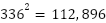 interactions per attention head. Although this sequence length remains computationally manageable, ProbSparse attention provides a structured mechanism to reduce redundant interactions and to evaluate whether selective long-range attention is beneficial for half-hourly load forecasting.
Nevertheless, the use of a Transformer-based architecture does not guarantee superior performance in a one-step-ahead forecasting task. Recent load observations may contain sufficient predictive information for CNN- or MLP-based models to remain competitive [31]–[38]. Therefore, this study does not assume that long-range dependencies are always necessary or that Informer is universally superior. Instead, it empirically investigates whether a seven-day historical window and an attention-based representation improve forecasting performance on the Tasmanian electricity demand dataset. This question is particularly relevant because the CNN baseline uses 48 historical observations, whereas Informer and MLP use 336 observations. Accordingly, the reported comparison reflects the combined effects of model architecture and model-specific historical context, and the results are interpreted as a dataset-specific evaluation rather than a strictly architecture-isolated comparison.
Existing studies commonly evaluate forecasting models using aggregate error measures such as mean absolute error, root mean squared error, and mean absolute percentage error. Although these metrics provide an overall assessment, they may conceal performance differences during rapid load transitions, high-demand periods, and isolated peak events. Computational cost is also important because a highly accurate model may not necessarily be the fastest or most suitable under all deployment constraints. A more informative assessment should therefore consider overall errors, high-load behavior, maximum-peak error, residual dispersion, prediction consistency, and computational time.
Based on this research gap, the present study evaluates an Informer-based deep learning model for one-step-ahead STLF using the TAS half-hourly electricity demand dataset from Tasmania, Australia. The forecasting task predicts demand for the next 30-minute interval using historical observations and calendar covariates. Informer is compared with CNN and MLP baselines, and all predictions are aligned with the same test period of 24,538 observations. This common evaluation period ensures consistency in metric calculation, although the model-specific input lengths are retained and explicitly acknowledged.
The research contribution is a dataset-specific, multi-perspective evaluation of Informer for one-step-ahead half-hourly electricity demand forecasting, rather than the introduction of a new Transformer architecture. The specific contributions are as follows:
- An Informer-based forecasting framework is implemented for one-step-ahead STLF using 122,736 half-hourly TAS observations, robust scaling, calendar covariates, and rolling evaluation.
- Informer is compared with CNN and MLP baselines over the same test period using MAE, MSE, RMSE, and MAPE, while transparently reporting the different historical input lengths used by the models.
- The evaluation extends beyond aggregate errors by examining the top-10% high-load subset, the single maximum-load point, forecast-error distributions, actual-versus-predicted consistency, and reported computational time.
- The study provides a balanced assessment of model strengths and limitations. Informer achieves the best overall and high-load-subset accuracy, while CNN performs better at the single maximum-load point and MLP requires the shortest reported runtime.
These contributions provide empirical evidence regarding the conditions under which attention-based long-sequence modeling is beneficial for Tasmania half-hourly load forecasting, while avoiding claims of universal superiority across datasets, forecasting horizons, or implementation environments [39]–[44].
RELATED WORK
Short-term electric load forecasting has been investigated using statistical, machine-learning, deep-learning, and Transformer-based approaches. Traditional statistical methods, including linear regression, autoregressive integrated moving average models, exponential smoothing, and Kalman filtering, remain attractive for their simplicity, interpretability, and relatively low computational cost. These methods can perform reliably when electricity-demand patterns are stable and can be represented by linear or weakly nonlinear relationships. However, their accuracy may deteriorate when load profiles become highly nonlinear, non-stationary, and affected by multiple temporal scales. Their performance also frequently depends on assumptions regarding stationarity, seasonality, and manually selected explanatory variables [45]–[50].
Machine-learning methods, such as support vector regression, random forests, gradient boosting, and ensemble learning, provide greater flexibility for representing nonlinear relationships. They can incorporate lagged demand, calendar indicators, and weather-related variables, but their effectiveness remains dependent on feature selection and input design. Consequently, the increasing availability of high-resolution smart-meter and electricity-market data has spurred the development of models that learn temporal representations directly from historical observations.
Deep-learning architectures have become widely used for this purpose. Multilayer perceptrons provide simple, computationally efficient nonlinear baselines, whereas convolutional neural networks extract local temporal features via convolutional filters. Long short-term memory and gated recurrent unit networks explicitly represent sequential dependencies. In contrast, hybrid architectures such as CNN–LSTM, CNN–GRU, and attention-enhanced networks combine local feature extraction, recurrent learning, and adaptive temporal weighting [51]–[58]. Nevertheless, recurrent models process observations sequentially, which may limit the degree of parallelization for long input sequences. CNNs primarily represent local structures unless their receptive fields are enlarged through deeper layers or larger kernels. In contrast, MLPs do not explicitly preserve temporal order unless the historical observations and calendar features are carefully organized.
Transformer-based forecasting models address some of these limitations by using attention mechanisms to model relationships among time steps. Informer introduces ProbSparse self-attention and a generative-style decoder to reduce the computational burden associated with conventional self-attention. Autoformer combines series decomposition with an auto-correlation mechanism, while FEDformer represents temporal patterns in the frequency domain. PatchTST divides historical sequences into patches and applies channel-independent modeling. TimesNet transforms one-dimensional time series into two-dimensional temporal representations, whereas iTransformer treats individual variables as tokens rather than time points [59]–[66]. These architectures demonstrate that Transformer-based forecasting can capture periodicity and long-range temporal relationships through different representation strategies.
However, the performance of Transformer-based models depends strongly on the dataset, forecasting horizon, sampling interval, input length, available covariates, and evaluation protocol. Their advantages are more evident in some long-horizon and long-sequence tasks. In contrast, simpler models may remain competitive for one-step-ahead forecasting because the most recent observations often contain strong predictive information. Therefore, the use of Informer for a 336-step input sequence should be evaluated empirically rather than justified solely by its theoretical efficiency. In this study, 336 half-hourly observations represent seven days of historical demand and contain both daily and weekly temporal contexts. ProbSparse attention is used to determine whether selectively modeling relationships within this historical window provides practical forecasting benefits for the next 30-minute interval.
Comparisons among forecasting architectures also require careful interpretation when different historical input lengths are used. A model supplied with a longer window receives more temporal information than a model trained on a shorter window, and any performance difference may therefore reflect both the architecture and the available historical context. In the present study, Informer and MLP use 336 observations, whereas CNN uses 48 observations according to the original saved experimental configurations. Accordingly, the comparison is conducted over an identical testing period and with common performance metrics. Still, it is interpreted as a comparison of complete model configurations rather than a strictly architecture-controlled experiment.
Another limitation of existing studies is their frequent reliance on aggregate measures such as mean absolute error, root mean squared error, and mean absolute percentage error. These metrics summarize average performance but may conceal model behavior during rapid transitions, high-demand periods, and isolated peak events. Such conditions are operationally important because large underestimations during peak demand may affect reserve allocation, generation scheduling, and grid reliability. Residual distributions and actual-versus-predicted scatter plots provide complementary evidence regarding error dispersion and consistency, while computational time helps characterize the practical cost of each implementation [67]–[70].
Within this context, the present study provides a dataset-specific, multi-perspective evaluation of Informer for one-step-ahead forecasting using the TAS half-hourly electricity demand dataset. Informer is compared with CNN and MLP baselines over the same test period of 24,538 observations. The evaluation includes overall forecasting metrics, top-10% high-load performance, error at the single maximum-load point, residual distributions, actual-versus-predicted agreement, and reported computational time. This design enables the strengths and limitations of Informer to be assessed more comprehensively and avoids interpreting aggregate accuracy as evidence of uniform superiority across all operating conditions.
PROPOSED METHOD
Problem Formulation
This study formulates short-term electric load forecasting as a one-step-ahead time-series regression problem. Let  denote the observed electricity demand at time step
 , where the data are recorded at 30-minute intervals. The objective is to predict the next demand value,
 , using a sequence of previous load observations and available temporal covariates. Therefore, the forecasting task can be expressed as learning a nonlinear mapping from historical electricity demand patterns to the next half-hour load value.
In general, the one-step-ahead forecasting function is defined as follows:
| 
| (1) |
where  is the predicted electricity demand at the next time step,
 is the look-back window length,
 represents known temporal covariates, and
 denotes the forecasting model learned from the training data. The historical load sequence provides information about recent consumption behavior, while the temporal covariates help the model capture periodic patterns related to time-of-day and calendar effects.
In this study, different input lengths are used according to the saved experimental configurations. The CNN baseline uses a look-back window of  , corresponding to one day of historical half-hourly load observations. In contrast, the Informer and MLP models use
 , corresponding to seven days of historical observations in the NeuralForecast configuration. This longer input window allows the Informer model to exploit both short-term variations and weekly temporal patterns. Although the models use different input lengths, their predictions are evaluated on the same test period to ensure a consistent comparison.
Thus, the forecasting problem in this paper is to estimate the next half-hour electricity demand as accurately as possible and to compare the ability of CNN, MLP, and Informer to learn the temporal relationship between historical TAS load values and future demand.
Proposed Informer-Based Forecasting Model
Informer is adopted as the main forecasting model in this study because it is designed for efficient long-sequence time-series forecasting. Unlike recurrent models that process temporal information sequentially, Informer uses an attention-based structure to directly model dependencies among historical time steps. This characteristic is suitable for half-hourly electricity demand forecasting, where both short-term load fluctuations and longer weekly consumption patterns may influence the next demand value.
For each forecasting time step , the input load sequence is defined as
| 
| (2) |
where denotes the observed electricity demand at time step , and is the input sequence length. In this study, the Informer model uses , corresponding to seven days of historical half-hourly load observations. In addition to the historical load sequence, calendar-based temporal covariates are also included and denoted as
| 
| (3) |
where represents known time-related features at time step . These covariates help the model capture recurring temporal patterns in daily and weekly electricity consumption.
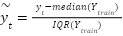
Before being used by the model, the load values are normalized using robust scaling to reduce the influence of extreme demand values. The scaled load value can be expressed as
| 
| (4) |
where  is the median value of the training load series, and
 is the interquartile range. This scaling strategy improves training stability, especially when the electricity demand series contains abnormal peaks or sudden changes.
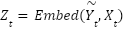
The scaled load sequence and temporal covariates are then embedded before being fed into the Informer encoder-decoder structure. The embedding process can be generally written as
| 
| (5) |
where  is the embedded input representation. This representation combines historical demand information and temporal covariate information into a latent feature space that the attention mechanism can process.
The core component of Informer is the attention mechanism. In the standard Transformer, scaled dot-product attention is calculated as
| 
| (6) |
where  ,
 , and
 are the query, key, and value matrices, respectively, and
 is the dimension of the key vectors. However, standard self-attention becomes computationally expensive when the input sequence is long. Informer addresses this issue using ProbSparse self-attention, which focuses only on the most informative query-key interactions. In a simplified form, the ProbSparse attention operation can be represented as (ProbSparse self-attention (PSSA)
| 
| (7) |
where  denotes the selected dominant queries. By reducing unnecessary attention computations, Informer can model long input sequences more efficiently than the standard Transformer.
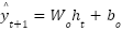
After the embedded sequence is processed by the Informer encoder-decoder layers, the final hidden representation is passed through a linear prediction head to generate the one-step-ahead forecast:
| 
| (8) |
where  is the final hidden representation learned by the Informer model,
 is the output weight matrix,
 is the bias term, and is the predicted electricity demand for the next half-hour interval.
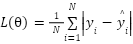
The model parameters are learned by minimizing the forecasting error between the actual and predicted load values. The training objective can be expressed using the mean absolute error loss:
| 
| (9) |
where  is the number of training samples,
 is the actual load value,
 is the predicted load value, and
 represents the trainable parameters of the Informer model.
In the final experimental configuration, the forecasting horizon was set to 1 step, corresponding to predicting electricity demand for the next 30-minute interval. The input size was set to 336 observations, representing seven days of historical half-hourly demand. The Informer model used a hidden size of 16, a convolutional hidden size of 32, and two attention heads. The model was trained using the mean absolute error loss, a learning rate of 0.001, and a maximum of 1,000 training steps. The validation loss was checked every 100 training steps, and early stopping was activated with a patience of five validation checks. Robust scaling and five calendar covariates were employed. The final Informer configuration contained approximately 8.9 thousand trainable parameters.
Baseline Models
To evaluate the forecasting effectiveness of the proposed Informer-based model, two deep-learning baselines are considered: a convolutional neural network (CNN) and a multilayer perceptron (MLP). These models represent two common neural forecasting strategies for short-term electric load forecasting. The CNN is used to extract local temporal features, whereas the MLP represents a feed-forward nonlinear forecasting approach.
The CNN baseline was implemented in TensorFlow/Keras using a supervised sliding-window architecture. Each forecasting sample contained the previous 48 half-hourly demand observations, corresponding to one day of historical information. The architecture consisted of one one-dimensional convolutional layer with 32 filters, a kernel size of 3, same padding, and the rectified linear unit activation function. A max-pooling layer with a pool size of 2 was applied to reduce the temporal dimension. The resulting feature maps were flattened and passed through a fully connected layer containing 32 rectified linear units, followed by a single linear output neuron. The model was trained for 100 epochs using the Adam optimizer with a learning rate of 0.001, mean squared error as the loss function, a batch size of 16, and a validation split of 0.2. The CNN contained 24,769 trainable parameters and did not use calendar covariates or input scaling.
The MLP baseline was implemented using NeuralForecast version 3.1.4, with a forecasting horizon of 1 step and an input size of 336 observations, corresponding to 7 days of half-hourly electricity demand. Five calendar covariates—hourminute, dayhour, weekday, monthday, and yearday-were included as future exogenous inputs. Because only the forecasting horizon, input size, and future exogenous variables were explicitly specified in the implementation, the remaining NeuralForecast defaults were retained. These defaults include two fully connected layers with 1,024 units per layer, rectified linear unit activation, mean absolute error loss, a learning rate of 0.001, a maximum of 1,000 training steps, a batch size of 32, identity scaling, and a random seed of 1. The resulting MLP contained approximately 3.1 million trainable parameters.
The three models do not use identical input lengths. The CNN receives 48 historical observations, whereas MLP and Informer receive 336 observations. Therefore, the comparison should be interpreted as an evaluation of the complete forecasting configurations rather than a strictly architecture-controlled comparison. The performance differences may be influenced by both the model architecture and the amount of historical information supplied to each model. To ensure consistency in the final evaluation, the predictions of all models are aligned with the same testing period of 24,538 observations, and the same actual load values and evaluation metrics are used.
Table 1 summarizes the main configurations of the evaluated models. The CNN focuses on local feature extraction from a one-day historical window. The MLP uses a seven-day input window and calendar covariates but does not explicitly model temporal relationships through convolution or attention. The Informer uses the same seven-day historical context as the MLP and additionally incorporates embedding layers, ProbSparse attention, an encoder–decoder architecture, and a linear prediction head. Consequently, the comparison evaluates the practical performance of local convolutional, feed-forward, and attention-based forecasting approaches under their original experimental configurations.
Table 1. Configuration Summary of the Evaluated Models
Model | Input length | Main configuration | Calendar covariates | Scaling | Loss | Trainable parameters |
CNN | 48 | Conv1D-32, MaxPooling1D, Flatten, Dense-32, linear output | No | None | MSE | 24,769 |
MLP | 336 | Two fully connected layers with 1,024 units per layer and linear output | Yes, five | Identity | MAE | Approximately 3.1 M |
Informer | 336 | Embedding, ProbSparse attention, encoder–decoder, linear output | Yes, five | Robust | MAE | Approximately 8.9 K |
Evaluation Metrics
The forecasting performance of the evaluated models is assessed using four commonly used regression metrics: mean absolute error (MAE), mean squared error (MSE), root mean squared error (RMSE), and mean absolute percentage error (MAPE). These metrics are selected because they provide complementary information on each model's forecasting accuracy.
MAE measures the average absolute difference between the actual and predicted load values. It is expressed in MW and provides a direct interpretation of the average forecasting error. MSE calculates the average squared error and imposes stronger penalties for large forecasting errors. RMSE is obtained by taking the square root of MSE, which converts the error magnitude back to the original unit of MW. MAPE measures the average relative forecasting error as a percentage of the actual demand, making it useful for comparing model performance in relative terms.
Let and denote the actual and predicted electricity demand values for the  -th test sample, respectively, and let be the total number of test samples. The evaluation metrics are defined as follows:
Proposed Informer-Based Forecasting Framework
Figure 1 illustrates the complete workflow of the proposed Informer-based framework for one-step-ahead short-term electric load forecasting. The framework consists of eight principal stages: data collection, data preprocessing, calendar-feature generation, forecasting configuration, Informer model construction, rolling evaluation, performance assessment, and result storage. This workflow provides a systematic description of how the raw Tasmanian electricity demand data are transformed into aligned forecasts and quantitative evaluation results.
As shown in Figure 1, the forecasting process begins with collecting the TAS electricity demand dataset from Tasmania, Australia. The dataset contains electricity-demand observations recorded at 30-minute intervals. During preprocessing, the SETTLEMENTDATE column is converted into a datetime format, while the TOTALDEMAND column is converted into a numeric target variable. Missing and duplicated observations are removed, the remaining records are arranged chronologically, and a unique series identifier is assigned. These operations ensure that the dataset has the continuous and correctly ordered structure required by the NeuralForecast framework.
After preprocessing, calendar-based temporal covariates are generated using the augment_calendar_df function. These covariates provide the model with information related to recurring temporal patterns in electricity consumption, particularly intra-day and weekly variations. The forecasting problem is then configured with a one-step-ahead horizon, corresponding to predicting electricity demand for the next 30-minute interval. The Informer input window contains 336 historical observations, representing seven days of half-hourly demand data. The validation and test sets contain 48 and 24,538 observations, respectively. Robust scaling is applied to reduce the influence of unusually high or low demand observations and improve numerical stability during model training.
The central stage of the framework is the Informer forecasting model. Historical electricity-demand observations and calendar covariates are first transformed into embedded representations. The Informer encoder processes these representations using a decoder architecture with ProbSparse attention. The attention mechanism identifies informative relationships within the seven-day historical sequence, while the encoder–decoder structure learns temporal representations that are relevant to the next forecasting interval. The resulting hidden representation is passed through a linear output layer to generate a one-step-ahead electricity demand forecast.
After model training, rolling evaluation is performed over the test period with a step size of one observation. At each evaluation step, the model generates a forecast for the next half-hour interval. The parameter refit = False indicates that the trained model is not retrained at every forecasting origin. Therefore, the rolling procedure evaluates sequential out-of-sample predictions while avoiding the additional computational cost of repeated model fitting. The forecast timestamps are subsequently aligned with the corresponding actual observations to ensure that all evaluation metrics are calculated from matched actual and predicted values.
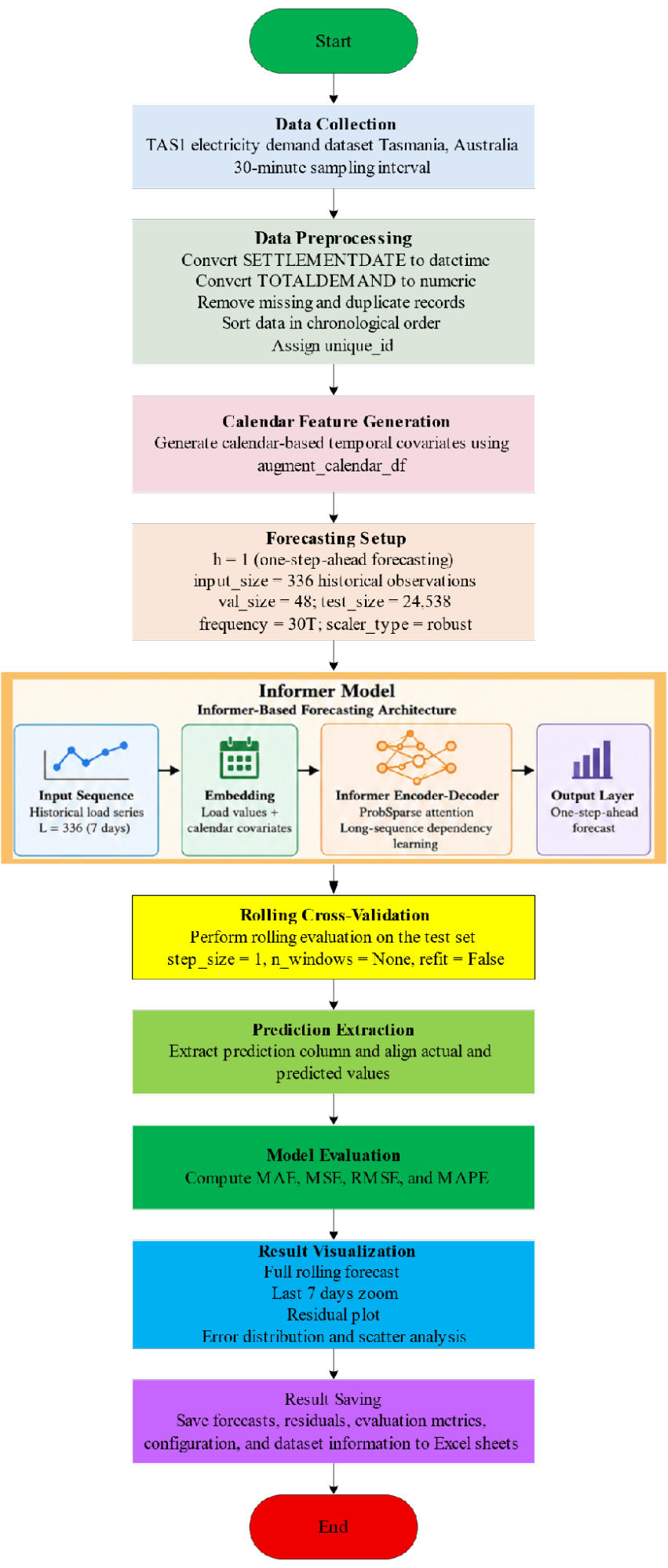
Figure 1. Flowchart of the proposed Informer-based short-term electric load forecasting framework
The aligned predictions are evaluated using mean absolute error, mean squared error, root mean squared error, and mean absolute percentage error. These metrics provide complementary assessments of average absolute error, sensitivity to large deviations, error magnitude in the original measurement unit, and relative percentage accuracy. Additional analyses include the complete rolling forecast, the forecast profile over the final seven days of the test period, residual behavior, error distributions, and actual-versus-predicted scatter plots. These graphical analyses provide further evidence regarding forecasting consistency, error dispersion, and model behavior across different demand levels.
Finally, the predicted values, actual observations, residuals, evaluation metrics, model configuration, and dataset information are exported to structured Excel worksheets. Saving these outputs improves the traceability of the experimental procedure and enables the reported numerical and graphical results to be independently checked. Overall, Figure 1 demonstrates that the proposed framework covers the complete forecasting process, from raw data preparation to model evaluation and result reporting, thereby supporting a clear and reproducible implementation of the Informer-based forecasting approach.
EXPERIMENTAL SETUP
This section presents the experimental design for evaluating the proposed Informer-based forecasting model and the two baseline models, namely CNN and MLP. The experiments were conducted on the TAS half-hourly electricity demand dataset. All models were evaluated using the same one-step-ahead forecasting horizon and the same final test period to ensure temporal alignment and metric consistency. However, because the original model configurations used different input lengths, scaling methods, covariates, loss functions, and software frameworks, the comparison should not be interpreted as a strictly architecture-controlled benchmark. The overall experimental setup includes data splitting, model configuration, training settings, and the final evaluation procedure.
Dataset Preparation and Data Splitting
This study uses the TAS electricity demand dataset, which represents half-hourly electricity load observations from Tasmania, Australia. The dataset contains two main columns: SETTLEMENTDATE and TOTALDEMAND. The SETTLEMENTDATE column records the timestamp of each observation, while the TOTALDEMAND column represents the electricity demand in MW. After converting the timestamp column into a datetime format, sorting the records chronologically, and removing invalid values, the final dataset contains 122,736 observations from 1 January 2015 00:30 to 1 January 2022 00:00. The electricity demand values range from 479.39 MW to 1,726.97 MW, with a mean value of 1,117.28 MW and a standard deviation of 150.09 MW.
Table 2 summarizes the main characteristics of the TAS electricity demand dataset used in this study. The dataset has a high temporal resolution, with one observation recorded every 30 minutes. Therefore, each day contains 48 load observations, making the dataset suitable for short-term electric load forecasting. The long historical period from 2015 to 2022 provides sufficient data to learn daily, weekly, and seasonal patterns of electricity consumption. In addition, the wide load range of 479.39 MW to 1,726.97 MW indicates that the dataset spans both low- and high-demand operating conditions, which is useful for evaluating the forecasting performance of different models across a range of load levels.
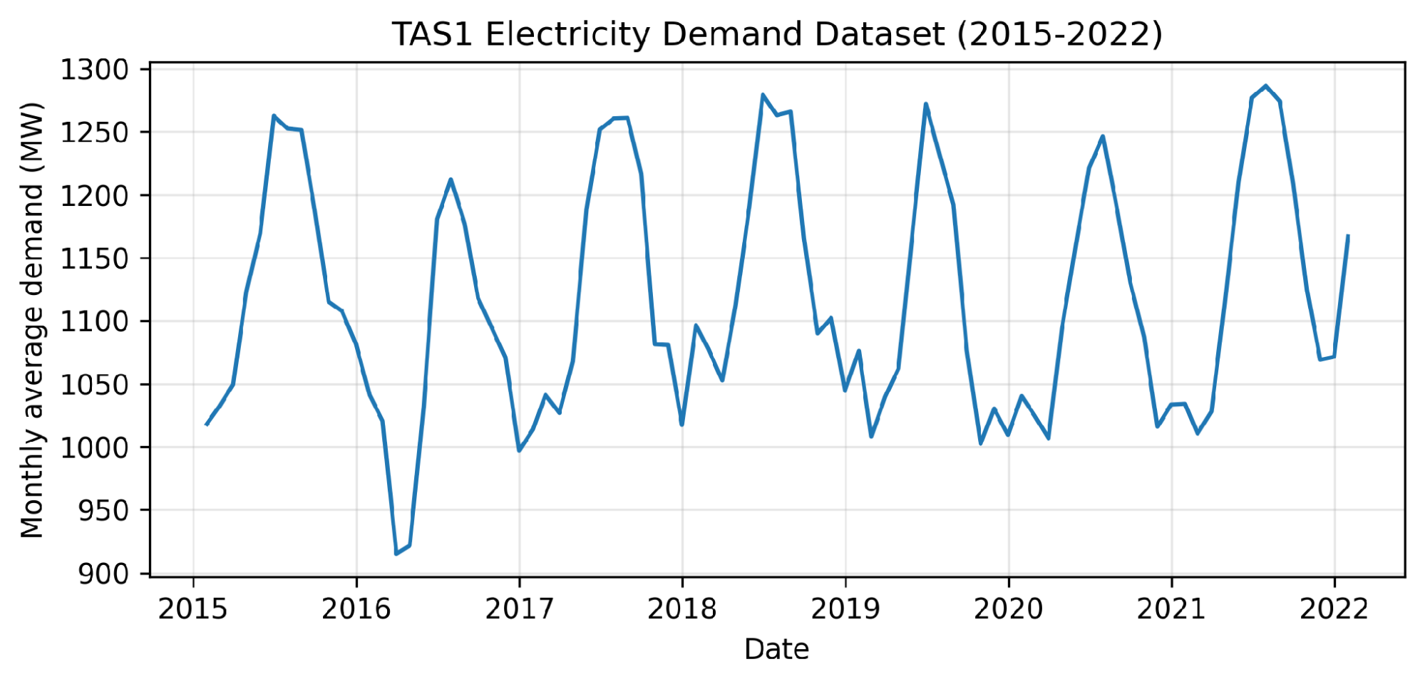
Figure 2 presents the monthly average electricity demand profile of the TAS dataset over the full study period. The curve shows clear temporal variations across different years, reflecting the non-stationary behavior of electricity consumption. Several recurring high-demand periods occur around the middle of different years, while average demand is lower during some transition periods. These variations indicate that the TAS load series contains seasonal and periodic characteristics. Therefore, the dataset provides a meaningful test case for evaluating whether the Informer model can capture both short-term fluctuations and longer temporal dependencies in half-hourly electricity demand data.
Before model training and evaluation, the raw TAS data were preprocessed to ensure a clean and consistent time-series structure. First, the SETTLEMENTDATE column was converted into a datetime format to preserve the correct temporal order of the observations. The TOTALDEMAND column was converted into a numeric load series measured in MW. The dataset was then sorted chronologically, and duplicated or invalid records were removed. This preprocessing step is important because time-series forecasting models rely strongly on the correct order and continuity of historical observations.
After data cleaning, calendar-based temporal covariates were generated to provide additional time-related information for the forecasting models. These covariates help the models capture recurring patterns associated with intra-day and weekly electricity consumption cycles. For the NeuralForecast-based models, including Informer and MLP, the forecasting configuration was set with a 30-minute frequency, a one-step-ahead forecasting horizon, and an input window of 336 historical observations. Since the data are recorded at 30-minute intervals, 336 observations correspond to seven days of historical load information. This longer input window allows the Informer and MLP models to learn both short-term load variations and weekly temporal patterns.
The CNN baseline was trained using a supervised sliding-window architecture with 48 previous half-hourly load values as input, corresponding to 1 day of historical observations. In contrast, the Informer and MLP models used an input length of 336 observations in the NeuralForecast rolling evaluation framework. This difference reflects the saved experimental configurations used in this study. Therefore, the model-specific input settings are clearly reported to ensure transparency and reproducibility.
The TAS dataset was arranged in chronological order before being split into training, validation, and test sets. Since electric load forecasting is a time-series prediction problem, random shuffling was not applied. This chronological splitting strategy ensures that the forecasting models are trained only on past observations and evaluated on future unseen data, which is consistent with real-world forecasting conditions. For the NeuralForecast-based models, the validation set comprised 48 observations, corresponding to 1 day of half-hourly data, while the test set comprised 24,538 observations. The CNN baseline predictions were aligned with the same testing period used by the Informer and MLP models.
The final testing period contained 24,538 half-hourly observations and was used as the common target period for CNN, MLP, and Informer. All saved predictions were aligned with the same actual demand timestamps before the evaluation metrics were recomputed. This procedure prevents performance differences from being caused by mismatched test periods or target observations. Nevertheless, the models use different input lengths, covariates, scaling methods, loss functions, and implementation frameworks. Therefore, the reported results represent a comparison of the complete implemented configurations rather than an isolated comparison of model architectures.
Table 2. Description of the TAS Electricity Demand Dataset
Property | Value |
Dataset | TAS electricity demand |
Region | Tasmania, Australia |
Time column | SETTLEMENTDATE |
Load column | TOTALDEMAND |
Sampling interval | 30 minutes |
Number of observations | 122,736 |
Date range | 2015-01-01 00:30 to 2022-01-01 00:00 |
Minimum load | 479.39 MW |
Maximum load | 1,726.97 MW |
Mean load | 1,117.28 MW |
Standard deviation | 150.09 MW |
Forecasting task | One-step-ahead STLF |
Figure 2. Monthly average electricity demand profile of the TAS dataset
Model Configuration
This study evaluates three forecasting models, including CNN, MLP, and Informer. Among them, the Informer model is selected as the primary proposed forecasting model, while CNN and MLP are used only as baselines for performance comparison. Therefore, the model configuration in this section mainly focuses on the proposed Informer architecture and its experimental settings.
The proposed Informer model is designed for one-step-ahead short-term electric load forecasting using the TAS electricity demand dataset. Since the dataset is recorded at 30-minute intervals, the forecasting horizon is set to h = 1, meaning the model predicts electricity demand for the next half-hour. The input size is set to 336 historical observations, corresponding to 7 days of past load data, since each day contains 48 half-hourly observations. This input length allows the model to use both recent load fluctuations and weekly historical patterns for forecasting.
The Informer model uses an attention-based architecture to capture temporal dependencies from long historical sequences. Its main components include embedding layers, ProbSparse attention, an encoder-decoder structure, and a linear prediction head. The embedding layers transform the input load sequence and calendar covariates into latent feature representations. The ProbSparse attention mechanism helps the model focus on the most informative time steps in the input sequence while reducing the computational burden of conventional self-attention. The encoder-decoder structure then learns the temporal relationships within the historical load sequence and generates the final one-step-ahead prediction through the linear output layer.
In addition to historical load observations, calendar covariates are included as temporal input features. These covariates provide useful time-related information, such as intra-day and weekly demand patterns. This is important for electricity load forecasting because demand behavior is often affected by repeated daily and weekly consumption cycles. Robust scaling is also applied to reduce the influence of abnormal or extreme load values and improve the stability of model training. The main configuration of the proposed Informer model is summarized in Table 3.
As shown in Table 3, the Informer model uses a 336-step input window to provide seven days of historical context for one-step-ahead forecasting. The configuration combines robust scaling, five calendar covariates, input embedding, ProbSparse attention, an encoder–decoder structure, and a linear prediction layer. This configuration enables the model to process both recent demand variations and recurring daily and weekly patterns. However, its empirical performance must be evaluated against the baseline configurations, as the input length, scaling method, covariates, and training procedures differ across models.
Table 3. Main configuration of the proposed Informer model
Parameter | Value | Description |
Main model | Informer | Primary forecasting model |
Framework | NeuralForecast 3.1.4 | Framework used to implement the model |
Deep-learning backend | PyTorch | Computational backend |
Forecasting horizon | 1 | Predicts the next 30-minute demand value |
Input size | 336 | Seven days of half-hourly observations |
Hidden size | 16 | Dimension of the hidden representation |
Convolutional hidden size | 32 | Hidden dimension of the convolutional component |
Number of attention heads | 2 | Number of parallel attention heads |
Loss function | MAE | Training objective |
Learning rate | 0.001 | Optimizer learning rate |
Maximum training steps | 1,000 | Upper limit of training iterations |
Validation check interval | 100 steps | Frequency of validation-loss evaluation |
Early-stopping patience | 5 validation checks | Stops training when validation performance does not improve |
Scaler type | Robust | Scaling applied to the Informer inputs |
Calendar covariates | 5 | hourminute, dayhour, weekday, monthday, and yearday |
Random seed | 1 | Default initialization seed |
Trainable parameters | Approximately 8.9 K | Model parameter count |
Main architecture | Embedding, ProbSparse attention, encoder–decoder, and linear output layer | Principal components |
Training Settings and Evaluation Protocol
The training settings were designed according to the one-step-ahead short-term load forecasting task. The forecasting horizon was set to h = 1, corresponding to predicting electricity demand for the next 30-minute interval. Since the TAS dataset is recorded at 30-minute intervals, this forecasting setting is consistent with the dataset's original sampling frequency.
The Informer and NeuralForecast MLP models used an input size of 336 observations, corresponding to seven days of historical half-hourly demand. Both models incorporated five calendar covariates and were evaluated using a validation set of 48 observations and a test set of 24,538 observations. However, their remaining configurations were different. Informer used robust scaling, a mean absolute error loss, a learning rate of 0.001, and a maximum of 1,000 training steps with early stopping. The MLP retained the NeuralForecast default identity scaling, mean absolute error loss, a learning rate of 0.001, and a maximum of 1,000 training steps without activated early stopping. The CNN used a 48-step input window, no calendar covariates, no explicit scaling, and mean squared error as its training loss. Therefore, the comparison represents the complete implemented configurations rather than a strictly architecture-controlled experiment.
The CNN baseline was trained using a supervised 48-step sliding-window structure. The model used 98,150 training samples and 24,538 testing samples obtained through a chronological 80:20 split with shuffle=False. The CNN was trained for 100 epochs using a batch size of 16 and a validation split of 0.2. Its forecasts were aligned with the same final 24,538 target observations used for the Informer and MLP evaluations. Although this procedure ensures temporal alignment of the reported metrics, the models receive different historical input lengths and use different covariate and scaling settings.
To ensure temporal alignment and consistent metric calculation, all models were assessed using the same final testing period. The reported metrics were recomputed from the saved and timestamp-aligned actual and predicted values rather than copied directly from model-specific summary outputs. The same aligned prediction rows were used to calculate the numerical metrics and generate the graphical analyses. This procedure ensures consistency in the evaluation targets, although the comparison remains configuration-specific because the evaluated models do not use identical inputs and training settings.
Implementation Environment
All experiments in this study were implemented in a Python-based computing environment using Google Colab. The runtime type was configured with Python 3, and GPU acceleration was enabled to support the training and evaluation of deep learning models. In this experiment, the Google Colab runtime was set to use an A100 GPU with high-RAM mode. This cloud-based environment provides sufficient computational resources to handle long historical input sequences and to perform rolling evaluation on the TAS half-hourly electricity demand dataset.
The Informer and MLP models were implemented using NeuralForecast version 3.1.4 with a PyTorch backend. The CNN baseline was implemented separately using TensorFlow/Keras. Consequently, the models were executed using different software frameworks and forecasting procedures. This distinction is important when interpreting the recorded elapsed times because framework initialization, data loading, model training, and rolling prediction may contribute differently to each reported value.
The Informer model was implemented using the Nixtla NeuralForecast library. The main modules used in the experiment included NeuralForecast for model management and forecasting execution, Informer for constructing the proposed forecasting model, MAE as the training loss function, and augment_calendar_df for generating calendar-based temporal covariates. These calendar covariates were used as future exogenous variables to provide additional time-related information for the forecasting model.
Data processing and numerical computation were performed using Pandas and NumPy. Pandas was used to read the TAS.csv file, convert the SETTLEMENTDATE column into a datetime format, format the TOTALDEMAND column as the target load series, remove invalid values, sort the dataset chronologically, and eliminate duplicate timestamps. NumPy was used for numerical operations and metric calculation. Matplotlib was used to visualize the actual and predicted load profiles, the zoomed forecasting results, and the residual series.
The TAS dataset was formatted according to the NeuralForecast framework's data structure. Specifically, the timestamp column was renamed as ds, the electricity demand column was renamed as y, and a unique_id column was added to identify the time series. The forecasting frequency in NeuralForecast was set to 30T, corresponding to the dataset's 30-minute sampling interval. Calendar features were generated using the Nixtla utility function and included in the Informer model as temporal covariates.
To reduce unnecessary runtime messages during model execution, logging outputs from Lightning Fabric and PyTorch Lightning were controlled. The rolling forecasting results, actual values, residuals, absolute errors, squared errors, percentage errors, evaluation metrics, model configuration, and dataset information were saved into an Excel file for further analysis and reporting. This implementation workflow ensured that the forecasting results were reproducible, traceable, and suitable for generating the numerical and graphical analyses presented in the results section.
As summarized in Table 4, the implementation environment was configured to support efficient and reproducible deep learning experiments. Using Google Colab with A100 GPU acceleration and high-RAM mode provided sufficient computational capacity to train the Informer model with long input sequences and rolling evaluation. In addition, the combination of Nixtla NeuralForecast, Pandas, NumPy, and Matplotlib enabled a complete workflow from data preprocessing and model training to forecasting evaluation and result visualization. By saving the prediction outputs, model configuration, and evaluation metrics into structured Excel sheets, the experimental process became more transparent and traceable. Therefore, the implementation environment used in this study ensured consistency, reproducibility, and reliability in evaluating the proposed Informer-based short-term load forecasting model.
Table 4. Implementation Environment and Software Tools
Item | Description |
Programming language | Python 3 |
Computing platform | Google Colab |
Hardware accelerator | NVIDIA A100 GPU |
RAM mode | High-RAM runtime |
NeuralForecast version | 3.1.4 |
Informer framework | NeuralForecast with PyTorch backend |
MLP framework | NeuralForecast with PyTorch backend |
CNN framework | TensorFlow/Keras |
Informer loss | MAE |
MLP loss | MAE |
CNN loss | MSE |
Data processing libraries | Pandas and NumPy |
Evaluation library | Scikit-learn and NumPy |
Visualization library | Matplotlib |
Calendar feature utility | augment_calendar_df |
Forecasting frequency | 30 minutes |
Output storage | Excel files containing forecasts, errors, metrics, configurations, and dataset information |
RESULTS AND DISCUSSION
To quantitatively compare the forecasting accuracy of the evaluated models, Table 5 presents the overall forecasting performance of MLP, CNN, and Informer on the common test set. The comparison is conducted using four evaluation metrics, including MAE, MSE, RMSE, and MAPE. MAE and RMSE measure the forecasting error in MW; MSE gives greater weight to large prediction errors; and MAPE evaluates the relative forecasting error as a percentage. Therefore, this table provides a comprehensive numerical assessment of each model's prediction accuracy.
Table 5. Overall Forecasting Performance on the Test Set
Model | MAE | MSE | RMSE | MAPE |
MLP | 29.3017 | 1447.8553 | 38.0507 | 2.6149 |
CNN | 21.2224 | 727.1635 | 26.9660 | 1.9231 |
Informer | 16.9317 | 536.0205 | 23.1521 | 1.5832 |
As shown in Table 5, the Informer model achieves the best overall forecasting performance among the three evaluated models. It yields the lowest error values across all metrics: MAE = 16.9317 MW, MSE = 536.0205, RMSE = 23.1521 MW, and MAPE = 1.5832%. In comparison, the CNN model achieves MAE = 21.2224 MW, MSE = 727.1635, RMSE = 26.9660 MW, and MAPE = 1.9231%. The MLP model produces the highest errors, with MAE = 29.3017 MW, MSE = 1447.8553, RMSE = 38.0507 MW, and MAPE = 2.6149%. These results indicate that Informer provides more accurate one-step-ahead electricity demand forecasts than both CNN and MLP on the TAS testing set.
The results in Table 5 show that the complete Informer configuration achieves lower aggregate forecasting errors than the evaluated CNN and MLP configurations on the TAS test set. However, the observed differences cannot be attributed exclusively to ProbSparse attention. Informer uses a 336-step historical window, five calendar covariates, robust scaling, and the MAE loss. The MLP uses the same input length and calendar covariates but retains identity scaling. In contrast, the CNN uses a 48-step input window without calendar covariates or scaling and is trained using the MSE loss. Therefore, Table 5 demonstrates the empirical advantage of the implemented Informer configuration rather than an architecture-isolated superiority of attention-based learning.
To further clarify the degree of improvement achieved by the proposed model, Table 6 presents the percentage error reduction of Informer compared with CNN and MLP. This analysis is important because the absolute metric values in Table 5 show which model performs better. At the same time, the reduction percentages in Table 6 quantify the improvement Informer achieves over the baseline models.
Table 6. Error Reduction of Informer Compared with Baseline Models
Comparison | MAE Reduction (%) | MSE Reduction (%) | RMSE Reduction (%) | MAPE Reduction (%) |
Informer vs. CNN | 20.22 | 26.29 | 14.14 | 17.67 |
Informer vs. MLP | 42.22 | 62.98 | 39.15 | 39.45 |
As shown in Table 6, Informer achieves clear error reductions compared with both CNN and MLP. When compared with CNN, Informer reduces MAE by 20.22%, MSE by 26.29%, RMSE by 14.14%, and MAPE by 17.67%. These results indicate that the proposed model improves not only the average absolute forecasting error but also the relative percentage error. The reduction in MSE also shows that Informer can decrease larger prediction deviations compared with CNN.
The improvement is larger when the complete Informer configuration is compared with the MLP configuration. Informer reduces MAE by 42.22%, MSE by 62.98%, RMSE by 39.15%, and MAPE by 39.45%. These reductions show that the implemented Informer configuration achieves substantially lower aggregate errors on the TAS test period. However, because Informer and MLP differ in scaling, architecture, parameter count, and training procedure, the improvement should not be attributed exclusively to attention-based temporal modeling.
Overall, Table 6 quantifies the reductions in aggregate forecasting error achieved by the complete Informer configuration relative to the evaluated CNN and MLP configurations. These reductions demonstrate better empirical performance on the common TAS testing period. Nevertheless, the experiment does not independently separate the effects of input length, calendar covariates, scaling, training loss, and model architecture. The percentage reductions should therefore not be interpreted as evidence that ProbSparse attention alone is responsible for the observed improvement.
After the quantitative results in Table 5 and Table 6 demonstrate Informer's forecasting advantage in error metrics, a visual evaluation is needed to examine how closely each model tracks actual load variation. Therefore, Figure 3 presents the actual and predicted load curves over the last seven days of the test set. This figure provides a direct comparison of the forecasting behavior of MLP, CNN, and Informer under short-term load fluctuations and repeated daily demand cycles.
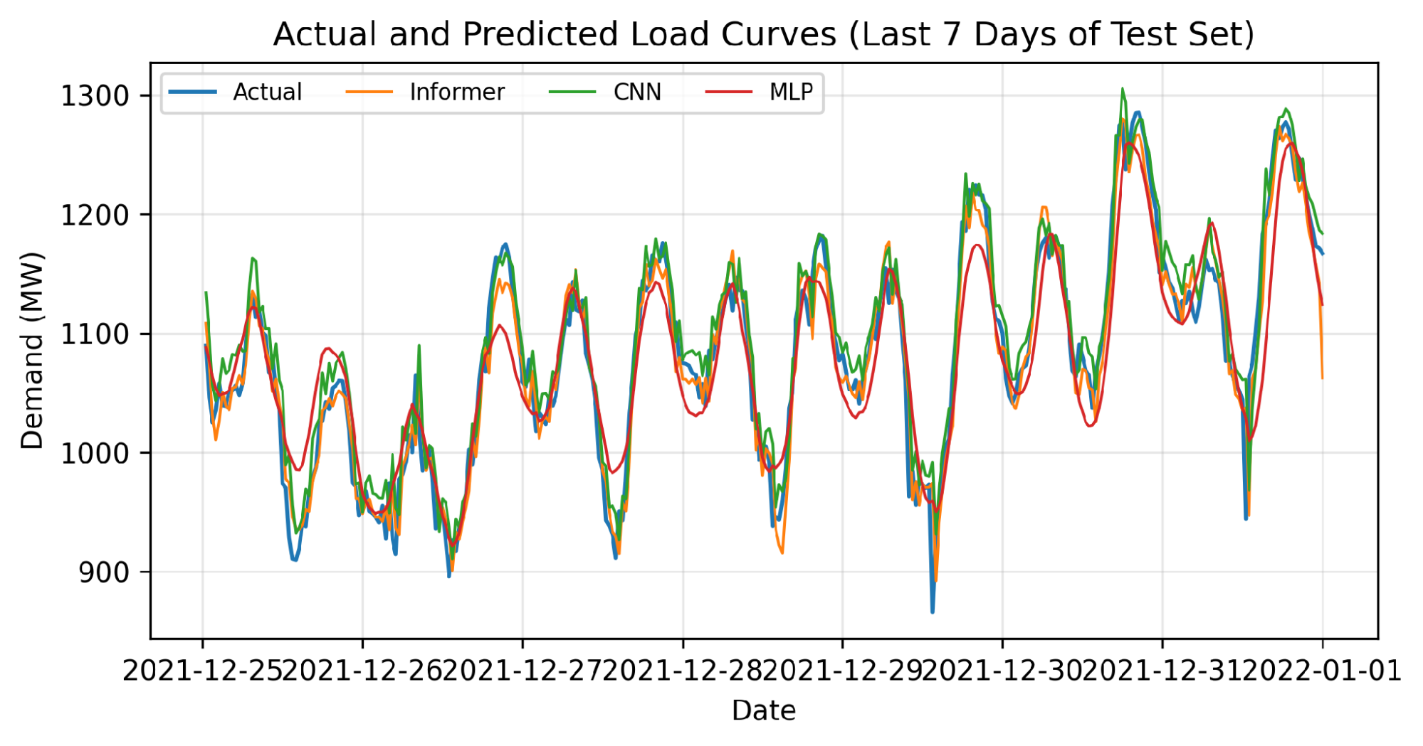
Figure 3. Actual and predicted load curves over the last seven days of the test set
As shown in Figure 3, the actual load curve exhibits clear daily fluctuations over the last seven days of the test period. Electricity demand repeatedly increases and decreases within each day, reflecting the short-term cyclic characteristics of half-hourly load data. All three models follow the general trend of the actual load profile, indicating that MLP, CNN, and Informer can learn the basic temporal patterns of the TAS demand series.
However, the degree of agreement differs among the evaluated models. The Informer prediction is generally closer to the actual load curve over most of the displayed period, which is consistent with its lower aggregate errors in Table 5 and Table 6. Nevertheless, visible deviations remain during several rapid load transitions and around some local peaks and valleys. Therefore, the graphical result indicates better overall tracking by the complete Informer configuration but does not imply that it eliminates localized forecasting errors.
For CNN, the model captures local load variations reasonably well, but some deviations persist around rapid transition regions and near peak or valley points. This may be because CNNs primarily exploit local temporal features within a short input window. In contrast, MLP exhibits more pronounced mismatches across several time intervals, particularly when the load changes abruptly. Since MLP mainly relies on nonlinear mapping through fully connected layers, it may have limited ability to explicitly represent the temporal order and dynamic structure of the load sequence.
Overall, Figure 3 shows that the implemented Informer configuration generally tracks the actual load profile more closely than the evaluated CNN and MLP configurations during the final seven days. This visual evidence supports the aggregate metric results and reveals remaining errors during abrupt demand changes.
After the visual comparison of the actual and predicted load curves in Figure 3, it is necessary to examine in more detail how the forecasting errors are distributed across the evaluated models. Therefore, Figure 4 presents the forecast error distribution of Informer, CNN, and MLP. This figure provides additional insight into the central tendency, spread, and stability of the prediction errors produced by the three models.
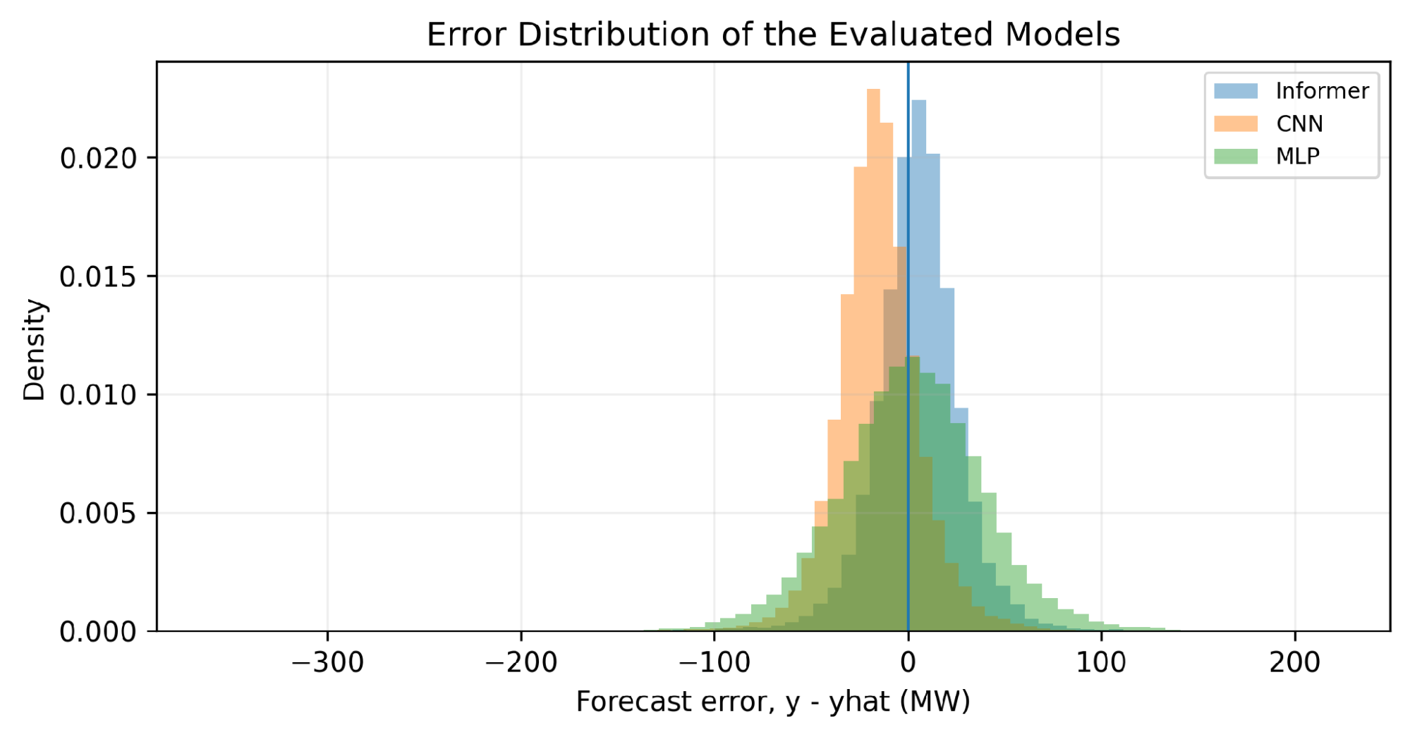
Figure 4. Forecast error distribution of Informer, CNN, and MLP
As shown in Figure 4, the forecast-error distributions of the evaluated models are centered near zero, indicating that large systematic shifts are not visually dominant in the displayed residual distributions. However, clear differences remain in the shape and spread of the distributions. The error distribution of Informer is more concentrated near zero and appears narrower than that of MLP, indicating that its prediction errors are generally smaller and more consistent. This result supports the numerical findings in Table 5 and Table 6, which show that Informer achieves the lowest overall forecasting errors among the evaluated models.
The CNN model also shows a relatively concentrated error distribution, but it is slightly shifted and still exhibits a wider spread than Informer in some regions. This suggests that CNN can provide reasonably accurate forecasts, yet its prediction errors are less stable than those of Informer. In contrast, the MLP model shows the broadest distribution among the three models, with errors spanning a wider range. Such a pattern indicates greater variability in prediction performance and confirms that the MLP is less effective at maintaining consistent forecasting accuracy over the test period.
Overall, Figure 4 shows that the implemented Informer configuration has a more concentrated empirical error distribution than the evaluated CNN and MLP configurations. This result is consistent with its lower MAE and RMSE values. However, a formal statistical test would be required to establish whether the differences in the error distributions are statistically significant.
After examining the distribution of forecasting errors in Figure 4, it is necessary to evaluate further how closely the predicted values match the actual electricity demand across the entire test set. Therefore, Figure 5 presents the scatter plots of the actual and predicted demand values for Informer, CNN, and MLP. This figure provides a visual assessment of the agreement, dispersion, and consistency of the forecasting results produced by the evaluated models.
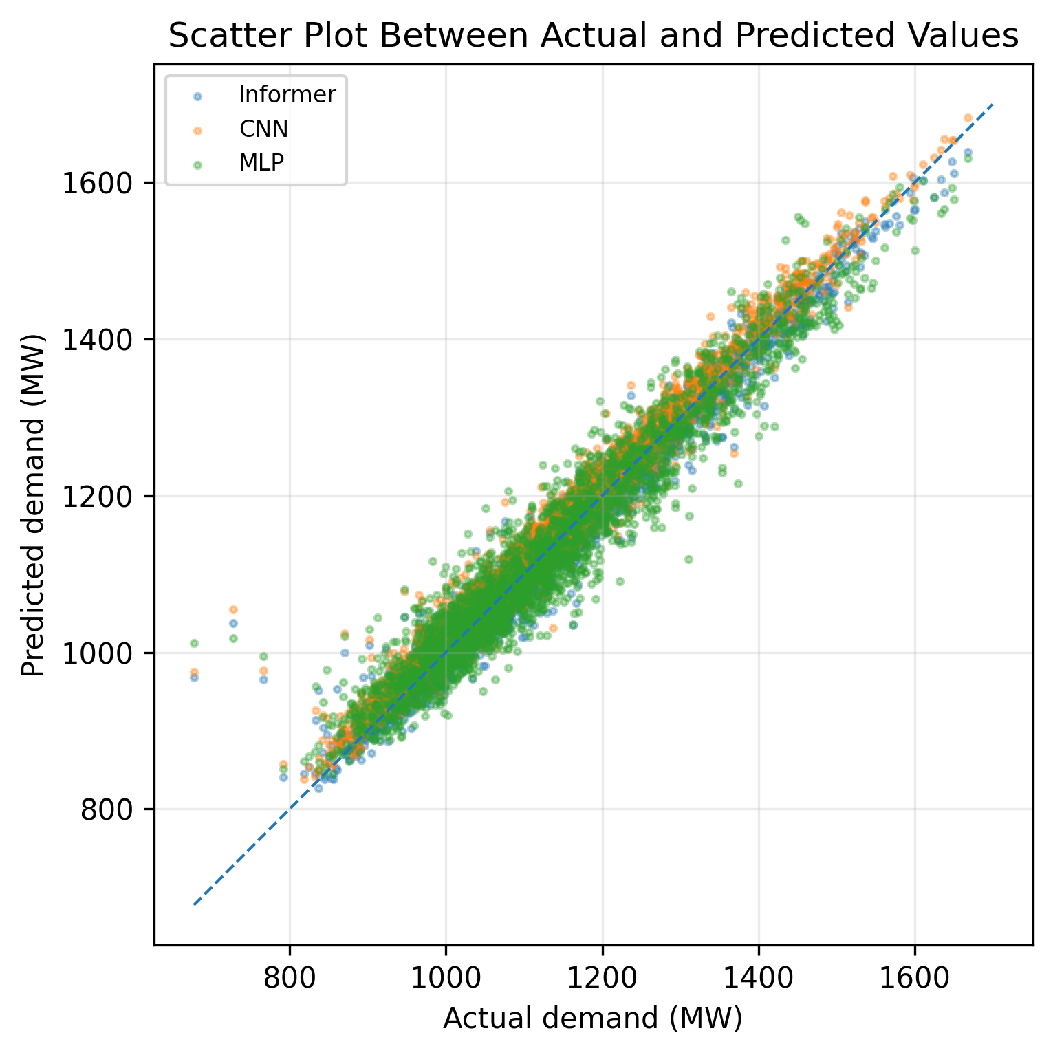
Figure 5. Scatter plot between actual and predicted demand values
As shown in Figure 5, most data points for the three evaluated models are distributed around the diagonal reference line, indicating that the predicted values are generally consistent with the actual electricity demand. This overall pattern confirms that all three models capture the main relationship between historical input information and target load values in the TAS dataset.
However, the degree of concentration around the diagonal line varies across models. The data points from Informer are generally more closely clustered around the ideal line, indicating stronger agreement between actual and predicted values. This result is consistent with the earlier findings in Table 5 and Table 6 and in Figure 3 and Figure 4, where Informer shows the lowest forecasting errors and the most concentrated error distribution. The tighter clustering suggests that Informer can provide more accurate and consistent predictions across a wide range of load levels.
The CNN model also shows relatively good alignment with the diagonal line, but its data points are slightly more dispersed across several load regions, especially as actual demand increases. This indicates that CNN can still produce competitive forecasts, but its predictive consistency is weaker than that of Informer. In contrast, the MLP model presents the widest dispersion among the three models. More points are distributed farther from the diagonal line, showing that MLP has larger deviations between predicted and actual values. This behavior further supports the conclusion that MLP is less effective in representing the temporal characteristics of the TAS demand series.
Overall, Figure 5 shows that the Informer predictions are more closely concentrated around the diagonal reference line over the observed test range. This finding is consistent with the lower aggregate errors reported for the complete Informer configuration. However, the scatter plot is descriptive and should not be interpreted as evidence of uniform superiority at every individual load level.
The scatter comparison in Figure 5 confirms the overall agreement between actual and predicted demand values across the full test set. However, in practical power system operation, forecasting accuracy during high-demand periods is especially important, as large errors under heavy load conditions can affect reserve scheduling, dispatch planning, and system reliability. Therefore, Table 7 presents the forecasting performance of MLP, CNN, and Informer under the top-10% high-load conditions, with a high-load threshold of 1344.876 MW.
Table 7. Forecasting Performance Under Top-10% High-Load Conditions (Threshold = 1344.876 MW)
Model | MAE | MSE | RMSE | MAPE |
MLP | 35.3446 | 2025.9204 | 45.0102 | 2.4707 |
CNN | 21.0558 | 683.4756 | 26.1434 | 1.4792 |
Informer | 19.4978 | 653.2280 | 25.5583 | 1.3646 |
As shown in Table 7, the Informer model achieves the best forecasting performance under high-load conditions. It obtains the lowest error values among the three evaluated models, with MAE = 19.4978 MW, MSE = 653.2280, RMSE = 25.5583 MW, and MAPE = 1.3646%. These results indicate that Informer maintains strong forecasting accuracy even when electricity demand is high.
Compared with CNN, Informer provides slightly better performance across all metrics. The MAE decreases from 21.0558 MW to 19.4978 MW, while the MAPE decreases from 1.4792% to 1.3646%. The reductions in MSE and RMSE also show that Informer can limit larger forecasting deviations more effectively during high-demand periods. This result shows that the complete Informer configuration maintains a small average advantage over CNN across the broader top-10% high-load subset. However, the observed difference cannot be attributed exclusively to the attention mechanism because the model configurations use different input lengths, covariates, scaling methods, and training procedures.
The advantage of Informer becomes more evident when compared with MLP. The MLP model records the largest errors, with MAE = 35.3446 MW, RMSE = 45.0102 MW, and MAPE = 2.4707%. This indicates that MLP has more difficulty following the load pattern during high-demand periods. The higher errors of the implemented MLP configuration indicate that it is less accurate over the selected high-load subset. Further controlled experiments would be required to determine whether this difference is caused by architecture, scaling, optimization, or other configuration choices.
Overall, the results in Table 7 demonstrate that Informer is more reliable than CNN and MLP under top-10% high-load conditions. This finding is important for short-term electric load forecasting because accurate prediction during high-demand periods can support more secure and economical power system operation. The lower MAPE of Informer indicates that the proposed model achieves better relative accuracy at high load.
After evaluating forecasting performance over the top-10% high-load samples in Table 7, it is also important to examine model behavior at the single maximum actual load point. Peak-load forecasting is critical to power system operation because large errors at the peak demand point can affect reserve planning, generation scheduling, and operational reliability. Therefore, Table 8 reports the forecasting error of each model at the maximum actual load point in the test set.
Table 8. Forecasting Error at the Maximum Actual Load Point
Model | Actual Peak | Predicted | Error | Absolute Error |
MLP | 1673.6700 | 1559.6516 | -114.0184 | 114.0184 |
CNN | 1673.6700 | 1645.2953 | -28.3747 | 28.3747 |
Informer | 1673.6700 | 1601.1365 | -72.5335 | 72.5335 |
As shown in Table 8, the maximum actual load in the test set is 1673.6700 MW. At this peak-load point, all three models underestimate the actual demand, as indicated by the negative error values. The MLP model predicts 1559.6516 MW, resulting in an error of -114.0184 MW and an absolute error of 114.0184 MW. The CNN model predicts 1645.2953 MW, producing the smallest absolute error of 28.3747 MW. The Informer model predicts 1601.1365 MW, with an error of -72.5335 MW and an absolute error of 72.5335 MW.
These results show that CNN provides the most accurate prediction at the single maximum actual load point. This finding is different from the overall results in Table 5 and Table 7, where Informer achieves the best performance across the full test set and under top-10% high-load conditions. The result suggests that CNNs may capture local peak behavior more effectively at this specific point, possibly because their convolutional structure focuses strongly on local temporal variations. However, this peak-load result is based on only one observation and should be interpreted as a complementary analysis rather than a complete measure of model performance.
The Informer model does not achieve the smallest absolute error at the maximum peak point, but it still performs better than MLP. More importantly, Informer remains the best model for overall forecasting accuracy and top-10% high-load forecasting performance. Therefore, Table 8 provides a more balanced interpretation of the evaluated models: Informer is the most accurate and stable overall, while CNN shows better predictions at the single maximum load point.
After examining the numerical high-load forecasting results in Table 7 and the peak-point forecasting errors in Table 8, a visual comparison is useful for more clearly highlighting the relative forecasting accuracy of the evaluated models under high-demand conditions. Therefore, Figure 6 presents the MAPE comparison of MLP, CNN, and Informer under the top-10% high-load conditions. This figure provides a direct visual summary of the relative percentage forecasting errors of each model when electricity demand is near high-load levels.
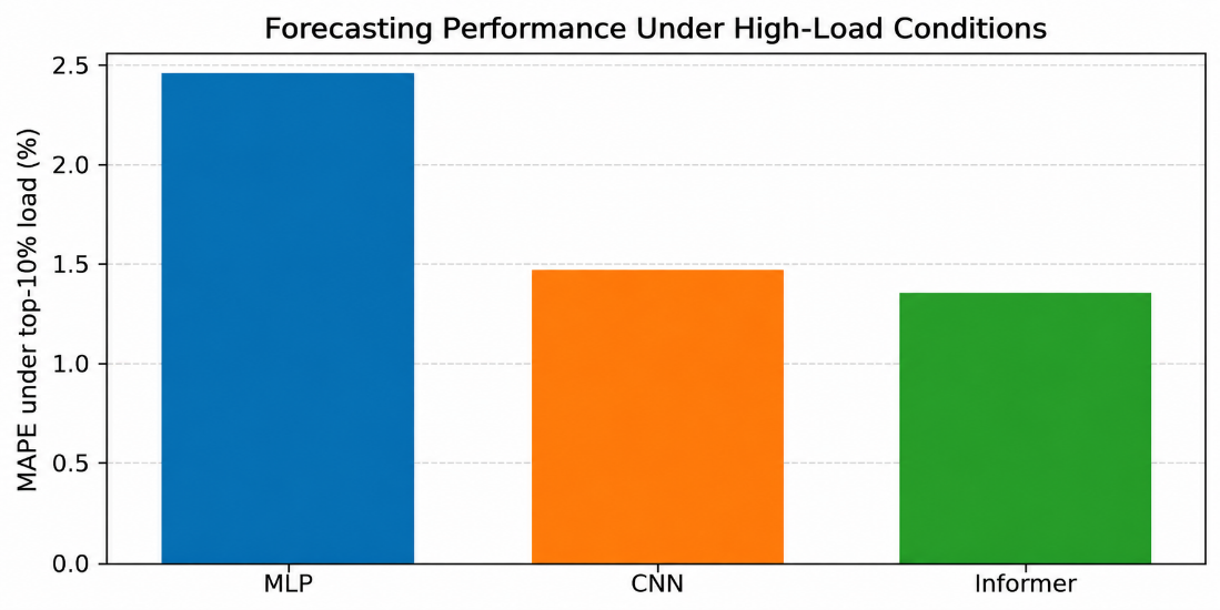
Figure 6. MAPE comparison under top-10% high-load conditions
As shown in Figure 6, the Informer model achieves the lowest MAPE among the three evaluated models under top-10% high-load conditions. Its MAPE is 1.3646%, which is lower than CNN's at 1.4792% and substantially lower than MLP's at 2.4707%. This result visually confirms the numerical findings reported in Table 7 and demonstrates that Informer provides the best relative forecasting accuracy during high-demand periods.
The figure also shows that the difference between Informer and CNN is relatively small, whereas both models produce substantially lower high-load MAPE values than MLP. This result indicates that the complete Informer configuration provides the best average relative accuracy over the top-10% high-load subset. However, because the evaluated configurations differ in input length, scaling, covariates, and loss functions, the observed advantage cannot be attributed solely to the attention mechanism. The higher MAPE of MLP indicates that its implemented configuration is less accurate under elevated demand conditions on this dataset.
Overall, Figure 6 strengthens the conclusion that Informer is the most reliable model under high-load conditions. Since forecasting accuracy during periods of high electricity demand is especially important for reserve scheduling, dispatch planning, and operational security, the lower MAPE of Informer underscores its practical value for short-term electric load forecasting.
After evaluating forecasting accuracy, the elapsed times recorded in the original experiments are reported in Table 9. These values provide descriptive information about the implemented forecasting procedures but do not represent a standardized architecture-level benchmark.
As shown in Table 9, MLP records the shortest elapsed time at 28.0330 s, followed by Informer at 75.5422 s and CNN at 1190.9676 s. However, the timing scopes are not identical. The CNN value primarily covers model construction and training in TensorFlow/Keras, whereas the NeuralForecast values include the rolling cross-validation procedure. In addition, the models use different frameworks, input lengths, scaling methods, losses, and forecasting procedures.
Table 9. Implementation-Specific Elapsed Times Recorded in the Original Experiments
Model | Reported Running Time (s) |
MLP | 28.0330 |
CNN | 1190.9676 |
Informer | 75.5422 |
Consequently, the reported times should be interpreted as implementation-specific measurements. They show that the evaluated Informer implementation required less elapsed time than the evaluated CNN implementation and more time than MLP, but they do not establish that Informer is inherently more computationally efficient than CNN. A controlled benchmark separating model-training time, total inference time, and per-sample prediction latency would be required for an architecture-level efficiency comparison.
After evaluating the computational time of the three models in Table 9, it is useful to provide a final visual summary of the main forecasting metrics. Therefore, Figure 7 presents a bar chart comparison of MAE, RMSE, and MAPE for MLP, CNN, and Informer. This figure visually highlights the relative forecasting performance of the evaluated models, using both absolute and percentage error measures.
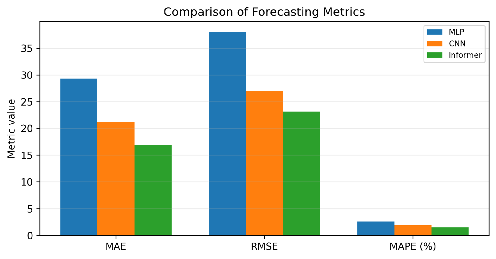
Figure 7. Bar chart comparison of MAE, RMSE, and MAPE for all evaluated models
As shown in Figure 7, the Informer model consistently achieves the lowest values across all three displayed metrics: MAE, RMSE, and MAPE. This visual result confirms the numerical findings previously reported in Table 5, where Informer outperforms CNN and MLP on the common test set. The lower MAE and RMSE values indicate that Informer produces smaller absolute forecasting errors, while the lower MAPE value indicates better relative forecasting accuracy.
The figure also shows that CNN performs better than MLP across all three metrics. Its bars are lower than MLP's for MAE, RMSE, and MAPE, indicating that the CNN provides more accurate predictions than the feed-forward baseline. However, the CNN bars remain higher than those of Informer, confirming that the complete Informer configuration achieves the strongest aggregate forecasting performance among the evaluated implementations.
The MLP model records the highest values for all three metrics, which visually reflects its weaker forecasting performance compared with the CNN and Informer models. This result is consistent with the previous analyses showing that MLP is less effective in capturing the temporal characteristics of the TAS electricity demand series. Since MLP mainly relies on fully connected nonlinear mapping, it may not model temporal dependencies as effectively as CNN and Informer.
Overall, Figure 7 provides a concise visual summary of the aggregate forecasting metrics. The lower MAE, RMSE, and MAPE values of Informer confirm that its implemented configuration achieves the best overall accuracy on the TAS test period. Because the evaluated configurations differ in several aspects, the figure supports the effectiveness of the complete Informer setup rather than isolating the individual contribution of ProbSparse attention.
Overall, the experimental results show that the complete Informer configuration achieves the lowest MAE, MSE, RMSE, and MAPE on the common TAS test period. The visual analyses are consistent with these aggregate results, showing closer overall tracking, a narrower empirical error distribution, and stronger actual-versus-predicted agreement than the evaluated CNN and MLP configurations. Under the top-10% high-load conditions, Informer also achieves the lowest average errors. However, CNN produces the smallest absolute error at the single maximum-load point, demonstrating that Informer's aggregate advantage does not extend uniformly to every extreme observation.
The reported elapsed times provide descriptive information about the original implementations but do not support an architecture-level computational-efficiency ranking because the models were implemented using different frameworks and timing scopes. Therefore, the principal conclusion of the experiment concerns forecasting accuracy rather than standardized computational superiority. The results support Informer as the strongest overall configuration in this dataset-specific evaluation while preserving a balanced interpretation of its peak-load limitations and experimental constraints.
CONCLUSION
This study evaluated an Informer-based deep-learning framework for one-step-ahead short-term electric load forecasting using the TAS half-hourly electricity-demand dataset from Tasmania, Australia. The proposed model was compared with CNN and MLP baselines over a common test period using MAE, MSE, RMSE, and MAPE. The evaluation was extended beyond aggregate accuracy to include top-10% high-load conditions, the single maximum-load point, residual distributions, actual-versus-predicted agreement, and computational time.
The results show that Informer achieves the best overall forecasting performance among the evaluated models, with MAE = 16.9317 MW, MSE = 536.0205, RMSE = 23.1521 MW, and MAPE = 1.5832%. Relative to CNN, Informer reduces MAE and MAPE by 20.22% and 17.67%, respectively. Relative to MLP, the corresponding reductions are 42.22% and 39.45%. Informer also achieves the lowest errors under the top-10% high-load conditions, indicating that its forecasting advantage is maintained across a broader set of high-demand observations.
The graphical analyses support these quantitative findings. Informer generally follows the actual load profile more closely, produces a more concentrated error distribution, and shows stronger agreement between actual and predicted values over the complete test set. However, CNN achieves the smallest absolute error at the single maximum-load point. This result demonstrates that the best aggregate model is not necessarily the most accurate model at every isolated extreme observation. Therefore, Informer should be regarded as the strongest overall model in this experiment rather than as uniformly superior under all operating conditions.
The recorded elapsed times show that MLP required the shortest time in the original experiments, followed by Informer and CNN. However, these values were obtained using different frameworks and timing scopes. The CNN value primarily covers TensorFlow/Keras model construction and training, whereas the Informer and MLP values include NeuralForecast rolling evaluation. Therefore, the reported times are implementation-specific and should not be interpreted as evidence of architecture-level computational superiority.
The main scientific contribution of this study is a dataset-specific and multi-perspective assessment of Informer for one-step-ahead half-hourly electricity-demand forecasting. The findings provide evidence that combining a seven-day historical input window, calendar covariates, robust scaling, and attention-based representation learning can improve aggregate and high-load forecasting accuracy on the TAS dataset. The study also contributes a more balanced evaluation by explicitly identifying conditions in which a simpler CNN remains competitive, particularly at the maximum-load point.
Several limitations should be acknowledged. First, the study uses a single regional electricity-demand dataset, and the conclusions cannot be generalized directly to other power systems. Second, CNN uses 48 historical observations, whereas MLP and Informer use 336 observations. Consequently, the comparison reflects both architectural differences and unequal historical information. Third, the forecasting models do not include weather, holiday, economic, or other external variables that may influence non-stationary demand behavior. Fourth, the analysis considers a one-step-ahead deterministic forecasting task and does not quantify predictive uncertainty. Finally, the reported runtime values are based on model-specific implementations and are not separated into standardized training and inference latency measurements.
Future research should evaluate all models under identical input windows, covariates, software settings, and hardware conditions to isolate architectural effects more clearly. The framework should also be validated on additional regional datasets and compared with recent forecasting architectures such as Autoformer, FEDformer, PatchTST, TimesNet, and iTransformer. Further extensions may incorporate weather and holiday variables, probabilistic forecasting, statistical significance testing, ablation analysis, transfer learning across regions, and multi-step-ahead forecasting. These directions would provide a more rigorous assessment of the scalability, robustness, and practical deployment potential of Informer-based load forecasting in real smart-grid environments.
REFERENCES
- Y. Eren and I. B. Küçükdemiral, “A comprehensive review on deep learning approaches for short-term load forecasting,” Renew. Sustain. Energy Rev., vol. 189, p. 114031, 2024, https://doi.org/10.1016/j.rser.2023.114031.
- K. Ullah, M. Ahsan, S. M. Hasanat, M. Haris, H. Yousaf, S. F. Raza, and Z. Ullah, “Short-term load forecasting: A comprehensive review and simulation study with CNN-LSTM hybrids approach,” IEEE Access, vol. 12, pp. 111858–111881, 2024, https://doi.org/10.1109/ACCESS.2024.3440631.
- A. L’Heureux, K. Grolinger, and M. A. M. Capretz, “Transformer-based model for electrical load forecasting,” Energies, vol. 15, no. 14, p. 4993, 2022, https://doi.org/10.3390/en15144993.
- H. Zhou, S. Zhang, J. Peng, S. Zhang, J. Li, H. Xiong, and W. Zhang, “Informer: Beyond efficient transformer for long sequence time-series forecasting,” Proc. AAAI Conf. Artif. Intell., vol. 35, no. 12, pp. 11106–11115, 2021, https://doi.org/10.1609/aaai.v35i12.17325.
- Z. Zhao, C. Xia, L. Chi, X. Chang, W. Li, T. Yang, and A. Y. Zomaya, “Short-term load forecasting based on the Transformer model,” Information, vol. 12, no. 12, p. 516, 2021, https://doi.org/10.3390/info12120516.
- J. W. Chan and C. K. Yeo, “A Transformer-based approach to electricity load forecasting,” Electr. J., vol. 37, no. 2, p. 107370, 2024, https://doi.org/10.1016/j.tej.2024.107370.
- S. H. Rafi, N. Al-Masood, S. R. Deeba, and E. Hossain, “A short-term load forecasting method using integrated CNN and LSTM network,” IEEE Access, vol. 9, pp. 32436–32448, 2021, https://doi.org/10.1109/ACCESS.2021.3060654.
- H. Eskandari, M. Imani, and M. P. Moghaddam, “Convolutional and recurrent neural network-based model for short-term load forecasting,” Electr. Power Syst. Res., vol. 195, p. 107173, 2021, https://doi.org/10.1016/j.epsr.2021.107173.
- M. N. Fekri, H. Patel, K. Grolinger, and V. Sharma, “Deep learning for load forecasting with smart meter data: Online adaptive recurrent neural network,” Appl. Energy, vol. 282, p. 116177, 2021, https://doi.org/10.1016/j.apenergy.2020.116177.
- M. N. Fekri, K. Grolinger, and S. Mir, “Distributed load forecasting using smart meter data: Federated learning with recurrent neural networks,” Int. J. Electr. Power Energy Syst., vol. 137, p. 107669, 2022, https://doi.org/10.1016/j.ijepes.2021.107669.
- D. Li, G. Sun, S. Miao, Y. Gu, Y. Zhang, and S. He, “A short-term electric load forecast method based on improved sequence-to-sequence GRU with adaptive temporal dependence,” Int. J. Electr. Power Energy Syst., vol. 137, p. 107627, 2022, https://doi.org/10.1016/j.ijepes.2021.107627.
- W. Yang, J. Shi, S. Li, Z. Song, Z. Zhang, and Z. Chen, “A combined deep learning load forecasting model of single household resident user considering multi-time scale electricity consumption behavior,” Appl. Energy, vol. 307, p. 118197, 2022, https://doi.org/10.1016/j.apenergy.2021.118197.
- P. P. Phyo and C. Jeenanunta, “Advanced ML-based ensemble and deep learning models for short-term load forecasting: Comparative analysis using feature engineering,” Appl. Sci., vol. 12, no. 10, p. 4882, 2022, https://doi.org/10.3390/app12104882.
- K. Wu, J. Wu, L. Feng, B. Yang, R. Liang, S. Yang, and R. Zhao, “An attention-based CNN-LSTM-BiLSTM model for short-term electric load forecasting in an integrated energy system,” Int. Trans. Electr. Energy Syst., vol. 31, no. 1, p. e12637, 2021, https://doi.org/10.1002/2050-7038.12637.
- Y. Wang, “An electricity load forecasting model based on multilayer dilated LSTM network and attention mechanism,” Frontiers in Energy Research, vol. 11, Art. no. 1116465, 2023, https://doi.org/10.3389/fenrg.2023.1116465.
- H. Bian, Q. Wang, G. Xu, and X. Zhao, “Load forecasting of a hybrid deep learning model considering accumulated temperature effect,” Energy Rep., vol. 8, pp. 205–215, 2022, https://doi.org/10.1016/j.egyr.2021.11.082.
- J. Cui, X. Zhang, F. Bi, C. Li, W. Kuang, K. Geng, and A. Bi, “Advanced short-term load forecasting with XGBoost-RF feature selection and CNN-GRU,” Processes, vol. 12, no. 11, p. 2466, 2024, https://doi.org/10.3390/pr12112466.
- S. M. Hasanat, M. Ahsan, K. Ullah, M. Haris, H. Yousaf, S. F. Raza, and Z. Ullah, “Enhancing short-term load forecasting with a CNN-GRU neural network with an attention mechanism,” IEEE Access, vol. 12, pp. 188791–188805, 2024, https://doi.org/10.1109/ACCESS.2024.3511653.
- X. Wen, H. Zhou, J. Liu, and Y. Zhang, “Deep learning-driven hybrid model for short-term load forecasting and smart grid information management,” Sci. Rep., vol. 14, p. 13632, 2024, https://doi.org/10.1038/s41598-024-63262-x.
- Y. Wang, “Short-term power load forecasting using SSA-CNN-LSTM,” Syst. Sci. Control Eng., vol. 12, no. 1, p. 2343297, 2024, https://doi.org/10.1080/21642583.2024.2343297.
- R. Zink, “Continual learning for very short-term load forecasting,” Appl. Energy, vol. 384, p. 126905, 2025, https://doi.org/10.1016/j.apenergy.2025.126905.
- R. Panigrahi, N. R. Patne, B. V. S. Vardhan, and M. Khedkar, “Short-term load analysis and forecasting using stochastic approach considering pandemic effects,” Electr. Eng., vol. 106, pp. 3387–3401, 2024, https://doi.org/10.1007/s00202-023-02135-4.
- O. Timur, “Short-term electric load forecasting for an industrial plant,” Energies, vol. 18, no. 5, p. 1144, 2025, https://doi.org/10.3390/en18051144.
- H. I. Beloev, “Short-term electrical load forecasting based on XGBoost,” Energies, vol. 18, no. 19, p. 5144, 2025, https://doi.org/10.3390/en18195144.
- M. J. Milovanović, M. M. Dragičević, N. R. Krečković, and B. D. Perović, “Short-term load forecasting with Taguchi-optimized single-layer feedforward neural networks: A MATLAB GUI,” ICCK Trans. Electr. Power Netw. Syst., vol. 1, no. 2, pp. 70–81, 2025, https://doi.org/10.62762/TEPNS.2025.295010.
- K. H. Baesmat and F. Shokoohi, “Evaluation of aggregate vs. appliance-level forecasting,” Smart Cities, vol. 8, no. 6, p. 199, 2025, https://doi.org/10.3390/smartcities8060199.
- J. Chen, “Short-term electricity load forecasting based on deep learning,” Appl. Sci., vol. 14, no. 14, p. 5966, 2024, https://doi.org/10.3390/app14145966.
- F. Guo, “A hybrid stacking model for enhanced short-term load forecasting,” Electronics, vol. 13, no. 14, p. 2719, 2024, https://doi.org/10.3390/electronics13142719.
- Q. Jiang, Y. Cheng, H. Le, C. Li, and P. X. Liu, “A stacking learning model based on multiple similar days for short-term load forecasting,” Mathematics, vol. 10, no. 14, p. 2446, 2022, https://doi.org/10.3390/math10142446.
- F. U. M. Ullah, N. Khan, T. Hussain, M. Y. Lee, and S. W. Baik, “Diving deep into short-term electricity load forecasting: Comparative analysis and a novel framework,” Mathematics, vol. 9, no. 6, p. 611, 2021, https://doi.org/10.3390/math9060611.
- H. Qiu, R. Hu, J. Chen, and Z. Yuan, “Short-term electricity load forecasting based on complete ensemble empirical mode decomposition with adaptive noise and improved sparrow search algorithm–convolutional neural network–bidirectional long short-term memory model,” Mathematics, vol. 13, no. 5, p. 813, 2025, https://doi.org/10.3390/math13050813.
- B. Chen and Y. Wang, “Short-term electric load forecasting of integrated energy system considering nonlinear synergy between different loads,” IEEE Access, vol. 9, pp. 43562–43573, 2021, https://doi.org/10.1109/ACCESS.2021.3066915.
- M. He, J. Zhang, and H. Wang, “A spatial-temporal attention network for short-term load forecasting of power systems,” Electr. Power Syst. Res., vol. 209, p. 107969, 2022, https://doi.org/10.1016/j.epsr.2022.107969.
- M. A. H. Akhand, S. Ahmed, M. A. Rahman, and M. M. H. Rahman, “Short-term load forecasting using deep learning and optimization techniques: A review,” Neural Comput. Appl., vol. 35, pp. 15463–15494, 2023, https://doi.org/10.1007/s00521-023-08448-4.
- M. F. H. Shiblee and P. Koukaras, “Short-term load forecasting in the Greek power system,” Energies, vol. 18, no. 19, p. 5060, 2025, https://doi.org/10.3390/en18195060.
- B. Magalhães, J. C. Ferreira, and J. S. Cardoso, “Short-term load forecasting based on optimized deep learning models,” Energies, vol. 17, no. 8, p. 1926, 2024, https://doi.org/10.3390/en17081926.
- Q. Cheng, Y. Zhang, and X. Liu, “Short-term load forecasting based on similar day theory and BWO-VMD,” Energies, vol. 18, no. 9, p. 2358, 2025, https://doi.org/10.3390/en18092358.
- B. W.-K. Yiu, T. Zhang, and C. W. Lee, “Short-term load forecasting using regularized greedy forest-based ensemble model,” IEEE Access, vol. 12, pp. 112426–112439, 2024, https://doi.org/10.1109/ACCESS.2024.3441642.
- H. H. Goh et al., “Multi-convolution feature extraction and recurrent neural network dependent model for short-term load forecasting,” IEEE Access, vol. 9, pp. 118528–118540, 2021, https://doi.org/10.1109/ACCESS.2021.3107954.
- B. Farsi, M. Amayri, N. Bouguila, and U. Eicker, “On short-term load forecasting using machine learning techniques and a novel parallel deep LSTM-CNN approach,” IEEE Access, vol. 9, pp. 31191–31212, 2021, https://doi.org/10.1109/ACCESS.2021.3060290.
- X. Ji, H. Huang, D. Chen, K. Yin, Z. Zuo, Z. Chen, and R. Bai, “A hybrid residential short-term load forecasting method using attention mechanism and deep learning,” Buildings, vol. 13, no. 1, p. 72, 2023, https://doi.org/10.3390/buildings13010072.
- S. Lu and T. Bao, “Short-term electricity load forecasting based on NeuralProphet and CNN-LSTM,” IEEE Access, vol. 12, pp. 84098–84112, 2024, https://doi.org/10.1109/ACCESS.2024.3407094.
- A. Mathew, R. K. Mehta, and S. K. Singh, “Medium-term feeder load forecasting and boosting peak accuracy prediction using the PWP-XGBoost model,” Electr. Power Syst. Res., vol. 237, p. 111051, 2024, https://doi.org/10.1016/j.epsr.2024.111051.
- Ş. Özdemir, Y. Demir, and Ö. Yildirim, “The effect of input length on prediction accuracy in short-term multi-step electricity load forecasting: A CNN-LSTM approach,” IEEE Access, 2025, https://doi.org/10.1109/ACCESS.2025.3540636.
- T. H. Nguyen et al., “Hybrid HHO-Wavenet model applies in short-term load forecasting for microgrid system,” in Proc. 6th Int. Conf. Green Technol. Sustain. Dev. (GTSD), pp. 1177–1183, 2022, https://doi.org/10.1109/GTSD54989.2022.9989027.
- O. Rubasinghe, X. Zhang, T. K. Chau, Y. H. Chow, T. Fernando, and H. H.-C. Iu, “A novel sequence-to-sequence data modeling based CNN-LSTM algorithm for three years ahead monthly peak load forecasting,” IEEE Trans. Power Syst., vol. 39, no. 1, pp. 1932–1947, Jan. 2024, https://doi.org/10.1109/TPWRS.2023.3271325.
- Y. Wang, N. Zhang, and X. Chen, “A short-term residential load forecasting model based on LSTM recurrent neural network considering weather features,” Energies, vol. 14, no. 10, p. 2737, 2021, https://doi.org/10.3390/en14102737.
- F. Rodrigues, C. Cardeira, J. M. F. Calado, and R. Melicio, “Short-term load forecasting of electricity demand for the residential sector based on modeling techniques: A systematic review,” Energies, vol. 16, no. 10, p. 4098, 2023, https://doi.org/10.3390/en16104098.
- B. Ibrahim and J. Rabelo, “Machine learning for short-term load forecasting in smart grids,” Energies, vol. 15, no. 21, p. 8079, 2022, https://doi.org/10.3390/en15218079.
- S. Akhtar, S. Shahzad, A. Zaheer, H. S. Ullah, H. Kilic, R. Gono, M. Jasiński, and Z. Leonowicz, “Short-term load forecasting models: A review of challenges, progress, and the road ahead,” Energies, vol. 16, no. 10, p. 4060, 2023, https://doi.org/10.3390/en16104060.
- G. Aquila, L. B. S. Morais, V. A. D. de Faria, J. W. M. Lima, L. M. M. Lima, and A. R. de Queiroz, “An overview of short-term load forecasting for electricity systems operational planning: Machine learning methods and the Brazilian experience,” Energies, vol. 16, no. 21, p. 7444, 2023, https://doi.org/10.3390/en16217444.
- M. D. Alanazi, “Enhancing short-term electrical load forecasting for sustainable energy management using a hybrid deep learning model,” Sustainability, vol. 15, no. 24, p. 16885, 2023, https://doi.org/10.3390/su152416885.
- M. Wood, “Day-ahead electric load forecast: A comprehensive LSTM-based approach,” Forecasting, vol. 5, no. 1, pp. 244–258, 2023, https://doi.org/10.3390/forecast5010016.
- Z. Huang, Y. Chen, and X. Wang, “Short-term load forecasting for regional smart energy systems,” Sustainability, vol. 16, no. 17, p. 7613, 2024, https://doi.org/10.3390/su16177613.
- W. Cao, Y. Liu, and J. Zhang, “Residential load forecasting based on long short-term memory neural networks,” Sustainability, vol. 16, no. 24, p. 11252, 2024, https://doi.org/10.3390/su162411252.
- Z. Yang, H. Liu, and Y. Li, “Forecasting very short-term power load with hybrid machine learning models,” Syst. Sci. Control Eng., vol. 13, no. 1, p. 2486136, 2025, https://doi.org/10.1080/21642583.2025.2486136.
- H. Li, J. Wang, and X. Zhou, “Short-term power load forecasting for integrated energy systems based on deep learning,” Front. Energy Res., vol. 12, p. 1384142, 2024, https://doi.org/10.3389/fenrg.2024.1384142.
- G.-F. Fan, Y.-Y. Han, J.-W. Li, L.-L. Peng, Y.-H. Yeh, and W.-C. Hong, “A hybrid model for deep learning short-term power load forecasting based on feature extraction statistical techniques,” Expert Syst. Appl., vol. 238, p. 122012, 2024, https://doi.org/10.1016/j.eswa.2023.122012.
- C. Yin and S. Mao, “Fractional multivariate grey Bernoulli model combined with improved grey wolf algorithm: Application in short-term power load forecasting,” Energy, vol. 269, p. 126844, 2023, https://doi.org/10.1016/j.energy.2023.126844.
- V. Ekambaram, A. Jati, N. Nguyen, P. Sinthong, and J. Kalagnanam, “TSMixer: Lightweight MLP-mixer model for multivariate time series forecasting,” in Proc—29th ACM SIGKDD Conf. Knowl. Discov. Data Mining, pp. 459–469, 2023, https://doi.org/10.1145/3580305.3599533.
- K. Benidis et al., “Deep learning for time series forecasting: Tutorial and literature survey,” ACM Comput. Surv., vol. 55, no. 6, pp. 1–36, 2022, https://doi.org/10.1145/3533382.
- A. Zeng, M. Chen, L. Zhang, and Q. Xu, “Are transformers effective for time series forecasting?” Proc. AAAI Conf. Artif. Intell., vol. 37, no. 9, pp. 11121–11128, 2023, https://doi.org/10.1609/aaai.v37i9.26317.
- C. Challu, K. G. Olivares, B. N. Oreshkin, F. G. Ramirez, M. M. Canseco, and A. Dubrawski, “N-HiTS: Neural hierarchical interpolation for time series forecasting,” Proc. AAAI Conf. Artif. Intell., vol. 37, no. 6, pp. 6989–6997, 2023, https://doi.org/10.1609/aaai.v37i6.25854.
- Z. Liu, H. Alavi, M. Li, and X. Zhang, “Self-supervised learning for time series forecasting: A review,” Knowl.-Based Syst., vol. 257, p. 109928, 2022, https://doi.org/10.1016/j.knosys.2022.109928.
- K. G. Olivares, C. Challu, G. Marcjasz, R. Weron, and A. Dubrawski, “NeuralForecast: User-friendly state-of-the-art neural forecasting models,” J. Open Source Softw., vol. 7, no. 79, p. 4570, 2022, https://doi.org/10.21105/joss.04570.
- P. Lara-Benitez, M. Carranza-Garcia, and J. C. Riquelme, “An experimental review on deep learning architectures for time series forecasting,” Int. J. Neural Syst., vol. 31, no. 3, p. 2130001, 2021, https://doi.org/10.1142/S0129065721300011.
- C. Sun, Y. Zhang, and H. Wang, “Graph neural network-based short-term load forecasting framework with dilated temporal convolution,” Data Sci. Eng., vol. 9, pp. 100–115, 2024, https://doi.org/10.1007/s41019-023-00233-8.
- D. Feng, D. Li, Y. Zhou, and W. Wang, “MLFGCN: Short-term residential load forecasting via graph attention temporal convolution network,” Frontiers in Neurorobotics, vol. 18, p. 1461403, 2024, https://doi.org/10.3389/fnbot.2024.1461403.
- C. Cai, Y. Wang, and X. Li, “Short-term load forecasting based on deep learning and multi-layer stacked bidirectional LSTM,” Appl. Sci., vol. 11, no. 17, p. 8129, 2021, https://doi.org/10.3390/app11178129.
- H. A. Al-Jamimi, M. A. Alotaibi, and A. K. Al-Othman, “Advancements in household load forecasting: Deep learning-based approaches and comparative analysis,” Electronics, vol. 12, no. 24, p. 4909, 2023, https://doi.org/10.3390/electronics12244909.
AUTHOR BIOGRAPHY
Tuan Anh Nguyen (One-Step-Ahead Half-Hourly Electricity Demand Forecasting in Tasmania Using an Informer-Based Deep Learning Model)