ISSN: 2685-9572 Buletin Ilmiah Sarjana Teknik Elektro
Vol. 8, No. 5, October 2026, pp. 1675-1699
A Hybrid Benchmark Framework for Metaheuristic Optimization across Cloud, Edge, Internet-of-Things, and Sixth-Generation Communication Networks
Hilal A. Fadhil 1, Shouket A. Ahmed 2, Maha I. Raheem 3, Mustafa Mohammed Al-Tuhafi 4,
Ahmed Dheyaa Radhi 5, Taha Almulaisi 6
1 Department of Electrical and Computer Engineering, Sohar University, Sohar, Oman
2 Department of Mechatronics Engineering Technologies, College of Engineering Technology, Al-Kitab University, Altun Kupri, 36001, Kirkuk, Iraq
3 College of Engineering, University of Information Technology and Communication, Al-Mansour, 3071, Baghdad, Iraq
4 Department of Medical Laboratory Techniques, Al-Bayan University, Baghdad, Iraq
5 College of Pharmacy, University of Al-Ameed, Karbala PO Box 198, Iraq
6 Renewable Energy Research Unit, Polytechnic College Hawija, Northern Technical University, Hawija, 36007, Iraq
ARTICLE INFORMATION |
| ABSTRACT |
Article History: Received 29 May 2026 Revised 17 October 2026 Accepted 07 November 2026 |
| 
Metaheuristics are the standard tool for NP-hard resource management across the cloud–edge–Internet-of-Things (IoT)–sixth-generation (6G) continuum, yet they are usually ranked on synthetic functions or a single application, so whether rankings transfer between problem classes is unknown. The research contribution is the Hybrid Benchmark Framework (HBF), a seeded engine that, unlike synthetic-only platforms such as the CEC suites, COCO/BBOB and IOHprofiler, places synthetic functions and communication–computing models behind a single continuous-encoding interface and statistical protocol, with a permutation test that quantifies ranking inversion. Five synthetic functions are combined with four seeded models of cloud scheduling, edge offloading, IoT clustering and 6G power allocation. Six optimizers (GA, PSO, GWO, WOA, DE and the 2026 Secant Optimization Algorithm) were run 20 times per problem with 9,030 evaluations each and compared with non-parametric tests, effect sizes and 95% confidence intervals. WOA and GWO hold the top two ranks on all five synthetic functions. On the three models that become categorical after decoding, the order reverses: the GA, last on the synthetic block, attains the best mean on all three, clearly on edge offloading (Hedges' g = 0.98, p < 0.001), whereas WOA falls to ranks 6, 6 and 4. Synthetic and categorical rankings are negatively correlated (Spearman ρ = −0.66, exact permutation p = 0.018), so pooled Friedman ranks cancel (p = 0.22). On the 6G model, which stays continuous after decoding, all optimizers lie within 0.028%. Optimizer rankings depend on the decoded objective's structure, so synthetic-suite results should be verified before discrete deployment. |
Keywords: Metaheuristic Optimization; Hybrid Benchmark Framework; Cloud–Edge–IoT Continuum; 6G Resource Allocation; Reproducibility |
Corresponding Author: Taha Almulaisi,
Renewable Energy Research Unit, Polytechnic College Hawija, Northern Technical University, Hawija, 36007, Iraq. Email: almalaisipi@gmail.com |
This work is open access under a Creative Commons Attribution-Share Alike 4.0 
|
Document Citation: H. A. Fadhil, S. A. Ahmed, M. I. Raheem, M. M. Al-Tuhafi, A. D. Radhi, and T. Almulaisi, “A Hybrid Benchmark Framework for Metaheuristic Optimization across Cloud, Edge, Internet-of-Things, and Sixth-Generation Communication Networks,” Buletin Ilmiah Sarjana Teknik Elektro, vol. 8, no. 5, pp. 1675-1699, 2026, DOI: 10.12928/biste.v8i5.16930. |
INTRODUCTION
Modern digital infrastructure is no longer organized around a single computing tier but around a continuum that stretches from centralized cloud data centers, through latency-sensitive edge and fog nodes, to massively distributed Internet-of-Things (IoT) devices, and increasingly to the radio fabric of sixth-generation (6G) communication networks [1]–[3]. Each layer of this continuum gives rise to resource-management decisions—how to map tasks to virtual machines, whether to offload a computation locally or to a server, which sensor should act as a cluster head, and how to divide transmit power among competing users—that are combinatorial, tightly constrained, and almost always NP-hard [4][5]. Because exact methods do not scale to the sizes encountered in practice, metaheuristic optimization has become the dominant solution paradigm across all four domains [6]–[10].
The last three years have witnessed an extraordinary proliferation of new metaheuristics. Bio-inspired, physics-inspired, human-inspired and mathematics-inspired optimizers such as the Coati Optimization Algorithm [11], the Dandelion Optimizer [12], the Mountain Gazelle Optimizer [13], the Hippopotamus Optimization Algorithm [14], the Electric Eel Foraging Optimization [15], and very recent mathematics-driven designs including the 2026 Secant Optimization Algorithm [16] have all reported state-of-the-art results on standard test suites. Comprehensive surveys [17]–[19] and benchmarking reviews [20][21] confirm both the pace of innovation and a growing unease about how these methods are evaluated.
This unease is well founded. The No-Free-Lunch theorem [22] establishes that, averaged over all possible problems, no optimizer can outperform any other; consequently, a claim of superiority is only meaningful relative to a clearly defined and representative set of problems.
In practice, however, two evaluation cultures coexist and rarely meet. The first relies on smooth, continuous synthetic functions (Sphere, Rastrigin, Ackley, Rosenbrock, Griewank, and the CEC suites), which are convenient, scalable and analytically understood but bear little resemblance to the discrete, constrained, plateau-ridden landscapes of real systems [20][21]. The second is a realistic but limited, hard to replicate and impossible to generalize, algorithm evaluation for a single, home-grown application (one scheduler, one offloading scenario, one slicing problem [1],[4],[23]). This leaves us with a literature where dozens of algorithms are labeled 'best' on incomparable testbeds, and in which reproducibility is the exception not the rule [21],[24]–[26].
Benchmarking infrastructure has matured in parallel. COCO/BBOB [27] and IOHprofiler [28] standardize performance assessment for black-box optimizers, the CEC competition suites supply the shifted and rotated functions on which most new algorithms, including SOA [16], are validated, and libraries such as MEALPY [29] and EvoX [30] make hundreds of optimizers and test functions available in a few lines of code. These platforms, however, evaluate optimizers on synthetic landscapes; none places models of communication and computing systems behind the same interface and statistical protocol, so none can show whether a ranking survives a change of problem class. Methodological guidelines [24][25] and evidence that the choice of benchmark set changes the conclusions [20],[31] make this gap consequential.
In this context, there are three key gaps in concrete terms. First, it is not possible to represent synthetic functions and realistic communication–computing problems in one optimization formulation, and then implement the same algorithm in both without modification. Second, there is very little cross-domain evidence; it is not at all clear whether or not an algorithm ranking that is achieved on smooth landscapes is maintained on combinatorial landscapes, or whether it is reversed. Third, there is hardly any tool that can be used to fix random seeds, release code and apply a standard statistical protocol [21],[26],[31] that is provided, making it easy to verify rankings published separately.
The rest of the paper is structured as follows. Section 2 describes work related to the subject of metaheuristics, their application in the four application areas and benchmarking practice. Section 3 details the framework architecture, the unified encoding and its analysis, the six optimizers and the four domain models. All the parameters for each optimizer and the experimental setup are described in Section 4. The results and a structured discussion of the main findings, the comparison with the previous studies, implications and the strengths and limitations of the study are presented within Section 5. Section 6 ends and summarizes further work.
This paper addresses those three gaps. The novelty lies not in proposing another optimizer but in constructing a hybrid, reproducible benchmark framework that measures how strongly algorithm performance depends on problem character across the cloud–edge–IoT–6G continuum. The research contribution is fourfold, and is stated below in measurable terms:
- C1 – Framework: HBF exposes nine problems, five synthetic functions and four seeded communication–computing models, through one continuous interface, so that each of the six optimizers runs on every problem without any problem-specific code; source code, seeds, instances and raw per-run results are archived and available from the corresponding author.
- C2 – Protocol: a paired design of 6 optimizers × 9 problems × 20 seeded runs (1,080 runs of 9,030 evaluations each), analyzed with the Friedman, Iman–Davenport, Nemenyi and Holm-corrected Wilcoxon procedures [26], effect sizes (Hedges' g, Vargha–Delaney
 , rank-biserial
 ) and 95% confidence intervals.
- C3 – Quantified inversion: a block-level inversion statistic with an exact permutation test, which shows that the synthetic and categorical rankings are negatively correlated (
 = −0.66, p = 0.018); the optimizer ranked first on all five synthetic functions (WOA) falls to ranks 6, 6 and 4 on cloud scheduling, edge offloading and IoT clustering, whereas the GA, last on the synthetic block, ranks first on all three. This gives the No-Free-Lunch theorem [22] an operational form for decoded problems.
- C4 – Mechanism: a band-crossing analysis of the unified encoding (3) to (4) that explains when an inversion should be expected, namely on piecewise-constant decoded objectives and not on continuous ones such as the 6G power split.
The research contribution is, in summary, a reproducible cross-domain benchmarking instrument, together with the quantified demonstration that optimizer rankings are conditional on problem class rather than universal, and with an explicit identification of the structural property of the problem — piecewise-constant objectives produced by discrete decoding — that determines when the inversion occurs.
Related Work
Metaheuristic Optimization Algorithms
Metaheuristics are problem-independent search strategies that balance exploration of the search space against exploitation of promising regions. The foundational population-based methods—the Genetic Algorithm [6], Particle Swarm Optimization [7] and Differential Evolution [10]—remain among the most widely used optimizers in engineering, and were later joined by a large family of swarm- and physics-inspired designs, including the Grey Wolf Optimizer [8] and the Whale Optimization Algorithm [9], which are surveyed and classified in [17],[19]. The most recent wave—Honey Badger [32], Snake [33], Coati [11], Dandelion [12], Mountain Gazelle [13], Reptile Search [34], Dwarf Mongoose [35], Hippopotamus [14], Electric Eel Foraging [15], RIME [36] and Crested Porcupine [37] optimizers, alongside human-inspired designs [38][39] and mathematics-inspired optimizers such as INFO [40] and SOA [16]—reflects an accelerating but increasingly crowded design space [17][18], and the metaphors behind many of these methods have been criticized for concealing operators that are close variants of earlier ones [41][42].
The Secant Optimization Algorithm (SOA), introduced in 2026 [16], is of particular interest because it departs from the bio-inspired metaphor and derives its update rule from the classical secant root-finding method, combining derivative-free secant steps for guided convergence with stochastic, expansion-factor sampling for global search. Its published validation is confined to continuous test suites (CEC 2020 and CEC 2021) and to continuous applications such as hyper-parameter tuning and photovoltaic parameter estimation [16]; its behavior on decoded, plateau-dominated combinatorial landscapes has not previously been reported. SOA is included for three checkable reasons: it was the most recent optimizer published in a peer-reviewed journal when the experiments were designed [16]; its update rule is derived from a numerical method rather than a natural metaphor, the design direction called for by recent critiques of metaphor-based metaheuristics [41][42] and shared with other mathematics-inspired optimizers such as INFO [40]; and its published validation is confined to continuous problems, so its behavior on decoded combinatorial models is an open question that the framework is built to test. No advantage of SOA on such models is assumed.
Metaheuristics Across the Cloud–Edge–IoT–6G Continuum
In cloud computing, metaheuristics are the standard tool for task scheduling and virtual-machine mapping, with recent work targeting makespan, energy and cost simultaneously [4],[23]; GA–PSO hybrids remain standard baselines in this setting, and standalone WOA has been reported to require hybridization before it becomes competitive on scheduling objectives [43][44]. At the edge, computation-offloading and load-balancing decisions are framed as latency–energy trade-offs solved with population-based search and surveyed extensively [1], and GWO-based frameworks have been proposed for collaborative edge offloading [45]. In IoT and wireless sensor networks, cluster-head selection and energy-aware routing dominate, where radio-energy models drive the objective and metaheuristics extend network lifetime [46]–[49]. In emerging 6G systems, network slicing and radio-resource allocation are increasingly optimized with learning-augmented and metaheuristic methods to maximize spectral efficiency under heterogeneous quality-of-service constraints [2],[3],[5],[50], the management, orchestration and integrated sensing-and-communication functions of 6G add further resource-allocation problems [51][52], and improved GWO variants have been applied to joint power control and user grouping in NOMA uplinks [53]. Across all four domains, however, each study optimizes a single problem with a handful of algorithms on its own testbed, which is precisely the fragmentation the present framework is designed to overcome.
Benchmarking Practice and Reproducibility
Recent research on benchmark choice [20] and review on test functions [21] report on a strong benchmark-dependency and the dependency on the number of function evaluations and the level of statistical reporting of the results. The recommended methodology—multiple independent runs, Friedman ranking, and Wilcoxon signed-rank tests—follows the now-classical guidance of Derrac et al. [26] and the later methodological guidelines of [24][25]. A 2026 particle-level study of exploitation behavior across the CEC 2025 suite [18] further argues that aggregate scores conceal the mechanisms that actually drive performance. Despite this, a framework that applies these statistical protocols uniformly across both synthetic and realistic communication-computing problems—with reproducible code—has been missing, motivating the contribution of this work.
General-purpose benchmarking platforms already exist, but none spans the synthetic and the communication–computing problem classes at the same time. COCO/BBOB automates the comparison of continuous optimizers and standardizes performance assessment through runtime distributions, yet its suites consist of analytic functions and contain no application-domain models [27]. IOHprofiler, with its analysis module IOHanalyzer, extends this idea through interactive fixed-target and fixed-budget analyses and covers pseudo-Boolean discrete problems in addition to continuous ones, but the discrete and continuous suites remain separate and neither is communication-oriented [28]. The CEC competition suites, on which most recent optimizers — including SOA [16] — are validated, are likewise purely synthetic, and Kudela [31] has shown that widely used synthetic sets can be structurally biased, so that rankings obtained on them may not be meaningful. At the opposite extreme, domain studies in cloud, edge, IoT and 6G optimize a single bespoke application with a problem-specific encoding [1]–[5],[23],[46]–[48],[50]. Table 1 positions the HBF against these alternatives; its distinguishing feature is not scale but coverage, namely one interface, one statistical protocol, and both problem classes within the same study.
Table 1. Positioning of the Hybrid Benchmark Framework with respect to representative benchmarking platforms and domain-specific optimization studies
Framework / study | Problem classes covered | Communication–computing domain models | Statistical protocol and code availability |
CEC competition suites [16],[21] | Synthetic continuous, shifted and rotated | None | Competition ranking; suite code released |
COCO / BBOB [27] | Synthetic continuous, single- and multi-objective | None | Runtime distributions; code released |
IOHprofiler / IOHanalyzer [28] | Synthetic continuous and pseudo-Boolean discrete, in separate suites | None | Fixed-target and fixed-budget statistics; code released |
Domain-specific optimization studies [1]–[5],[23],[46]–[48],[50] | One bespoke application per study | One domain per study | Reported inconsistently; code rarely released |
Benchmarking reviews [20][21],[31] | Survey of existing suites | Discussed, not implemented | Recommendations only |
MEALPY [29] | Library of optimizers; test functions supplied separately | None | No prescribed protocol; code released |
EvoX [30] | Numerical benchmark suites and neuroevolution tasks, GPU-accelerated | None | Scalable execution; no prescribed protocol; code released |
HBF (this work) | Five synthetic functions and four domain models in one suite | Cloud, edge, IoT and 6G | Friedman, Iman–Davenport, Nemenyi CD, Holm-corrected Wilcoxon, effect sizes, 95% CIs and an inversion test; seeds, generators, raw results and code archived |
THE HYBRID BENCHMARK FRAMEWORK
Framework Architecture
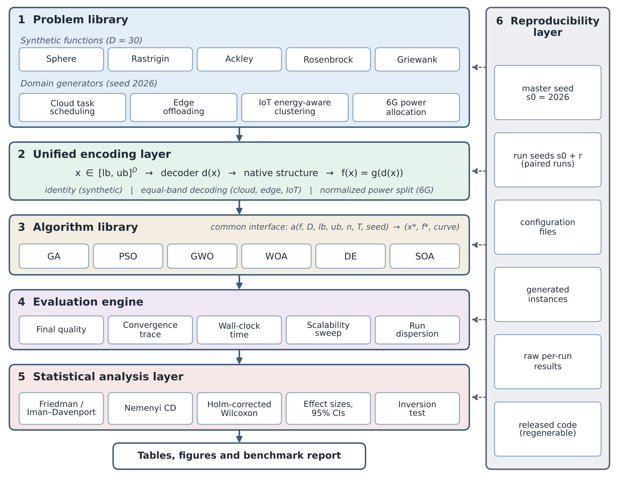
The HBF is structured as a multi-level evaluation system as indicated in Figure 1. A problem library exposes both synthetic functions and real world domain functions, a unified encoding layer maps each possible candidate solution from a common continuous vector to the native structure of each problem, a library of algorithms hosts the six optimizers as interchangeable, plug-and-play minimizers, an evaluation engine measures quality, convergence, runtime and scalability, a statistical analysis layer computes Friedman ranks and Wilcoxon tests, effect sizes, confidence intervals, the inversion statistic and win counts, and a reproducibility layer fixes random seeds, configurations and datasets for every reported number to be reproduced. That's the reason that a single implementation of one algorithm can be tested and modified on the smooth Sphere function as well as on the constrained 6G power-allocation problem.
Figure 1. Layered architecture of the Hybrid Benchmark Framework (HBF): five processing layers (left) and the reproducibility layer that records every seed, configuration, instance and raw result (right)
Figure 2 shows the evaluation pipeline as it is executed. A single configuration fixes the master seed (2026), the population size, the iteration budget and the number of runs. The problem library is instantiated once with that seed (Step 1), so every optimizer faces identical instances, and each problem is wrapped in the unified encoding (Step 2) before the six optimizers are registered behind one interface (Step 3). Steps 4 and 5 form the inner loop: each algorithm–problem–run triple takes its seed from the shared family s0 + r, which pairs the runs across algorithms, and the evaluation engine records the final value, the convergence trace and the wall-clock time. The scalability sweep (Step 6) repeats this loop on cloud scheduling at five instance sizes. Steps 7–9 run once per experiment: the statistical layer applies the tests of Section 3.6, the reporting layer produces every table and figure in Section 5, and the reproducibility layer stores seeds, configurations, instances and raw results.
Algorithm 1 gives the same workflow as pseudocode. Lines 1–4 instantiate and wrap each problem once; lines 5–14 run the paired experiment and store the mean, standard deviation and 95% confidence interval of each algorithm–problem pair; lines 15–17 rank the algorithms and apply the Friedman, Nemenyi and Holm-corrected Wilcoxon procedures; line 18 runs the scalability sweep; and lines 19–20 persist and report the results. Because the only algorithm-specific element is the call in line 9, adding an optimizer or a problem changes no other line.
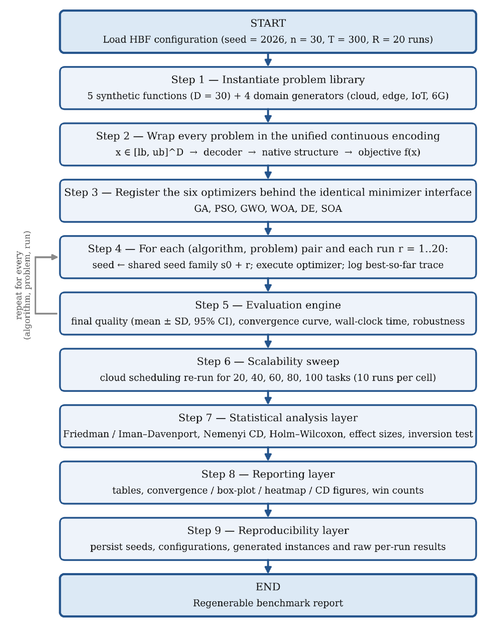
Figure 2. Flowchart of the HBF evaluation pipeline, from configuration loading to the regenerable benchmark report; the loop of Steps 4–5 is repeated for every algorithm, problem and run
Algorithm 1: HBF evaluation workflow Input: problem library P (5 synthetic + 4 domain models), algorithm library A (6 optimizers), population n = 30, iterations T = 300, runs R = 20, master seed s0 = 2026 Output: quality, convergence, runtime and statistical reports 1 for each problem p in P do 2 instantiate p with seed s0 # fixed instance, identical for all algorithms 3 wrap p in the unified encoding of Eq. (2) # continuous x -> native structure -> f(x) 4 end for 5 for each algorithm a in A do 6 for each problem p in P do 7 for r = 1 to R do 8 seed <- s0 + r # shared seed family: comparisons are paired 9 (x*, f*, curve) <- a(f_p, D_p, lb_p, ub_p, n, T) 10 record f*, curve and wall-clock time 11 end for 12 store mean, standard deviation and 95% confidence interval over the R runs 13 end for 14 end for 15 rank algorithms per problem (1 = best); compute average Friedman ranks 16 apply the Friedman test of Eq. (23); if significant, compute the Nemenyi critical difference 17 apply pairwise Wilcoxon signed-rank tests; adjust the p-values by the Holm procedure 18 repeat steps 5-14 on cloud scheduling for 20, 40, 60, 80 and 100 tasks (scalability sweep) 19 persist seeds, configurations, generated instances and raw per-run results 20 return tables, figures and statistical summary |
The framework consists of  decision variables and each problem is stated as the minimisation of an objective function over a box-constrained continuous domain (1).
| 
| (1) |
The vector – it is the central object in the design, and the synthetic functions will directly use the vector, while the domain problems will pass it to a decoder that will convert the continuous coordinates into discrete decisions for the structure, as described in Section 3.2 and in (2).
Unified Continuous Encoding
The performance of continuous optimizers on an inherently discrete problem is evaluated using a uniform decoding rule, without changing the internals of the continuous optimizers. If the variable to select from among M categories (a virtual machine for a task, an offloading tier, or a cluster-head flag), the unit interval of these categories is subdivided into M equal bands as in (2), and the normalized coordinate is represented by an integer index.
| 
| (2) |
The same logic can be used for the assignment of tiers for the offloading of edges (3 bands), selection of binary cluster-head based on a threshold, and normalization of power split for 6G allocation. The search space experienced by each optimizer is well defined, and the objective mimics the discrete cost of the engineering problem being solved; both the mapping and the target have deterministici characteristics, with a bounded search space.
There are only two properties that justify this decoding rule. First, it is measure preserving; that is, each of the M categories is given an interval of width  , and a uniformly initialised population leads to a uniform distribution on the discrete alternatives, with no favouring of any category in advance. Second, the composite objective
 , where d is the decoder and g the native discrete cost, is deterministic and bounded and repeated evaluations of the same continuous point will always result in the same value, while the search problem is well-posed. The drawback of these properties is that f is piecewise constant: d is constant on the interior of every band, and thus f has zero gradient almost everywhere, and only changes at the
 band boundaries of each variable.
This is a piecewise-constant structure that imposes a bias which needs to be explicitly stated since it is not a neutral structure among the optimizers examined here. Small continuous displacement operators, like the spiral operator WOA and the encircling operator GWO, and the velocity update operator PSO at the end of a run, are often used and their offspring fall within the same band as their parent, do not generate enough information to change the solution decoded and do not change the objective. These operators with large or recombinative jumps (the GA's blend crossover and the scaled difference vectors in DE) tend to cross band boundaries more often, and thus explore the discrete space more effectively.
The encoding is thus a part of the ranking inversion reported in Section 5.4, and not just the algorithms themselves. It does not try to eliminate this effect, since it is this interface that makes it possible to compare the results from across the domains: the effect is stated here, it is obvious in the domain results and is identified in Section 5.6.4 as the motivation for introducing native discrete operators, which would enable the encoding contribution to be separated by ablation.
An analytical statement of the size of this effect is possible. Let  be a categorical variable whose normalized coordinate xi is broken down into
 equally-sized subintervals of width , and an operator that shifts
 by
 such that |
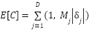
 . If the parent is uniformly distributed in its own band, then the probability of the category switching is (3) and for a dimensional move the expected value of the number of variables whose decoded value switches is (4).
| 
| (3) |
| 
| (4) |
The step-length dynamics of each optimizer is connected with its success on the decoded models in (4). The distance moved by each individual is a multiple of the distance to the current leader or leaders, scaled by a coefficient that decreases as a linear function of distance to leader,  falls to zero and more evaluations return the same objective as the population shrinks. Gaussian mutation with a fixed standard deviation keeps
 bounded below for the GA, and the difference vectors of DE scale with the spread of the population, which
 preserves for longer. The effect should be strongest for WOA, whose spiral and shrinking-encircling moves both scale with the distance to a single leader. On the 6G model no band quantization is applied, so every displacement changes the objective and (4) places no constraint on the search; this model therefore serves as a control on which no inversion is expected Section 5.2. A second bias is ordinal: equal bands place category 1 next to category 2 but far from category M, although virtual machines and offloading tiers have no natural order, so small moves can reach only neighboring categories. Both effects are recognized in the literature on continuous metaheuristics for discrete problems, where the decoding or binarization rule has been found to affect performance more than the transfer function [54][55].
The structure results in the computational complexity of the framework. The main experiment requires 6 algorithms × 9 problems × 20 runs = 1,080 runs, and each of the 6 optimizers requires  arithmetic on a population of size
 in dimensions, making
 = 9,030 arithmetic operations per run (with n = 30 and
 = 300). The decoding step adds
 for the cloud and edge models, whose objectives are obtained by a single pass over the tasks, and
 for the 6G model if the per-user rates of 22 are evaluated independently. The IoT clustering model is the most expensive, because every non-cluster-head node must be matched to its nearest head, which is
 in the number of nodes in the worst case, with
 = 50 here. The statistical layer is negligible by comparison, requiring
 to rank k algorithms on
 problems plus
 pairwise tests. The framework therefore scales linearly in the number of algorithms, problems and runs, which is what keeps the full protocol cheap enough to be regenerated end to end.
The population is stored as fitness values, which for  and
 use up ~24 kB of double precision memory, and the convergence trace uses
 memory, with T being the number of iterations, while the node-distance matrix used in the IoT model has an memory requirement if it is precomputed; memory does not limit the framework at the sizes studied here.
Synthetic Benchmark Functions
The unimodal Sphere of (5), the highly multimodal Rastrigin of (6), the Ackley function of (7), the narrow-valley Rosenbrock function of (8) and the Griewank function of (9) anchor the synthetic side of the suite. They vary in unimodal, multimodal and partly separable structure and their global optimum and difficulty are analytically known, which makes them suitable stress tests for exploration and exploitation [21]. All functions have global minimum value  at
 except Rosenbrock which has a global minimum at
 . The search range of every coordinate is [−100, 100] for Sphere, [−5.12, 5.12] for Rastrigin, [−32, 32] for Ackley, [−30, 30] for Rosenbrock and [−600, 600] for Griewank.
Optimization Algorithms
Six minimizers are implemented behind an identical interface that receives the objective, dimension and bounds and returns the best position, best value and convergence trace. Five are well-established baselines and one is the 2026 Secant Optimization Algorithm.
The composition of this pool is deliberate rather than exhaustive. GA, PSO and DE are the three most widely used population-based methods in the cloud, edge and IoT optimization literature surveyed in Section 2.2, while GWO and WOA are the two swarm optimizers most frequently reported as state of the art on continuous engineering benchmarks [8][9]. Together they supply four distinct search mechanisms — recombination-based, velocity-based, difference-vector-based and leader-based — which are exactly the operator families that the unified encoding stresses differently, and SOA adds a mathematics-inspired mechanism that belongs to none of them. Restricting the pool to six keeps the full factorial protocol, together with the scalability sweep, small enough to be regenerated end to end from the archived code, which is a requirement of the reproducibility objective rather than a limitation of the interface: adding an optimizer requires no change to the problems or to the statistics, and Section 5.6.4 identifies enlargement of the pool as the primary planned extension.
Genetic Algorithm (GA)
The real-coded GA [6] applies tournament selection, blend ( ) crossover and Gaussian mutation with elitist replacement, maintaining diversity through recombination of high-quality parents—an operator set that, as the results will show, is particularly effective on the discrete domain problems.
Particle Swarm Optimization (PSO)
PSO [7] moves each particle under cognitive and social attraction toward its personal best and the global best, as given by the velocity and position updates of (10) and (11); a linearly decaying inertia weight shifts the search from exploration to exploitation over the run.
| 
| (10) |
| 
| (11) |
Grey Wolf Optimizer (GWO)
GWO [8] models a social hierarchy in which the three best wolves (alpha, beta, delta) guide the pack; each agent encircles the leaders through the distance and step relations of (12) and is repositioned at their average according to (13), with the control parameter decreasing linearly from two to zero.
| 
| (12) |
| 
| (13) |
Whale Optimization Algorithm (WOA)
WOA [9] switches between the best solution and a logarithmic-spiral bubble-net maneuver (which is described by (14), with a probability switch and a decreasing coefficient resulting in the high exploitation that makes WOA a winner on the smooth functions in this study.
| 
| (14) |
Differential Evolution (DE)
DE [10] is based on trial vectors generated by subtracting a scaled difference between two randomly selected individuals in the population from a third (DE/rand/1 mutation in (15), binomially crossover and greedy selection ( = 0.5 and
 = 0.9).
| 
| (15) |
Secant Optimization Algorithm (SOA, 2026)
In SOA [16] there is a change from the biological metaphor to a mechanism based on the secant root-finding algorithm. They each calculate a secant step from their fitness gap to the global best as in (16) with a small constant to prevent a divide by zero, and add adaptive guidance to the best and second-best references plus a term motivated from stagnation awareness for exploration to get the position update of (17). The weight and amplitude of the exploited terms are respectively the cosine and linear schedules of (18), which cause this search to change from global sampling to local refinement as the iterations go on. The procedure is summarized in Algorithm 2.
Algorithm 2: Secant Optimization Algorithm (minimization) Input: objective f, dimension D, bounds [lb, ub], population n, iterations T Initialize population X uniformly in [lb, ub]; evaluate fitness Identify global best g and second-best s for t = 1 to T do a <- 2 (1 - t/T) # exploration amplitude w <- 0.5 (1 + cos(pi t / T)) # exploitation weight (Eq. (18)) for each agent i do s_i <- secant step from f(x_i), f(g) # Eq. (16) clip s_i to +/- 0.5 (ub - lb) x_i <- x_i + w r1 (g - x_i) + (1-w) r2 (s - x_i) - 0.5 a r3 s_i # Eq. (17) with probability a/4: x_i <- g + a (rand - 0.5)(ub - lb) # exploration clip x_i to [lb, ub] evaluate fitness; update g and s end for return g, f(g), convergence curve |
Real-World Domain Problem Models
There are four repeatable domain generators that map a continuous vector to a meaningful communication-computing task.
Three checks define the validity of these generators and should accompany any use of the framework; all three are implemented in the generator-check routine of the code and were run on the instances used in this study. (i) Structural validity: every decoded solution must satisfy the native constraints of its domain. All 1,000 random solutions drawn for each model decoded to a valid structure, with every task assigned to exactly one virtual machine or tier and every 6G power split summing to the 10 W budget; the cluster-head range of the IoT model, which is enforced through the penalty of (21), was satisfied by 119 of the 120 final IoT solutions, the exception being one PSO run that ended with nine cluster heads and is reported with its penalty included. (ii) Determinism: instantiating each generator twice with seed 2026 gave identical objective values on 200 random solutions. (iii) Non-degeneracy: the goal of the random solutions should be different from the standard constructive heuristic: longest-task-first/ minimum-completion-time list scheduling for cloud model; greedy tier assignment, starting with all the tasks at the edge and gradually moving one task at a time while the objective improves for edge offloading; and equal power allocation for 6G. The mean objective of random solutions and the heuristic value were 58.81 and 27.85 for cloud scheduling, 421.07 and 176.89 for edge offloading, 45.58 and 18.06 mJ for IoT clustering, and −248.19 and −260.20 for 6G allocation, so every landscape carries information rather than being flat. The heuristics also serve as reference points: the best optimizer mean improves on the heuristic for edge offloading, IoT clustering and 6G allocation, but on cloud scheduling list scheduling (27.85) is better than every optimizer, including the best one (28.60), a result discussed in Section 5.6.4.
Cloud Task Scheduling
Forty independent tasks are mapped onto eight virtual machines of differing processing speed and power consumption. The objective of (19) combines the makespan M, defined as the maximum machine completion time, with a load-imbalance penalty and an energy term, so that a good solution must be simultaneously fast, balanced and energy-aware rather than optimal on any single criterion. In the instance used here, task lengths  are drawn uniformly from 1,000–10,000 million instructions, machine speeds
 from 500–2,000 MIPS and busy-state powers
 from 0.1–0.3 kW;
 is the busy time of machine
 ,
 the standard deviation of the busy times,
 = 0.5 and
 = 0.05, and each coordinate is decoded into one of = 8 machines by (2).
| 
| (19) |
Edge computation offloading
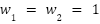
Forty tasks are distributed to local devices, edge servers, and cloud: The different tiers have different processing speeds and bandwidths for transmitting the tasks. The goal of (20) takes into consideration the overall latency but also penalizes for any deadline breaches, reflecting the fundamental latency–energy tradeoff in edge computing [1]. Each coordinate is decoded into one of = 3 tiers (local, edge, cloud). Input sizes are drawn uniformly from 1–10 Mb, workloads from 0.5–5 Gcycles and deadlines di from 1–4 s; local devices compute at 1 GHz, the edge (20 GHz) and cloud (60 GHz) processors and their uplinks (100 and 50 Mbps) are shared equally among the tasks assigned to them, and cloud execution adds a propagation delay of 0.2 s. The latency  is the sum of transmission and computing time, the energy ei is that of local computing at 0.9 W or of transmission at 0.5 W, and
 and
 .
| 
| (20) |
IoT Energy-Aware Clustering
The 50 sensor nodes are spread over a square field, and a threshold is used on every coordinate to select the cluster heads, the remaining nodes join the nearest cluster head and the total transmission energy of (21) is obtained using the standard first-order radio model, but including a penalty to ensure that the number of cluster heads remains in a valid range [46]–[48]. The nodes are placed uniformly in a 100 m × 100 m field with the base station at (50, 175) m. A node is a cluster head when its coordinate is at least 0.5, and every node sends a  = 4,000-bit packet over the distance di to its nearest cluster head or, if it is a cluster head, to the base station, with
 = 50 nJ/bit and
 = 10 pJ/bit/
 ;
 is the distance of the number of cluster heads from the admissible range of 2–8,
 , and the objective is expressed in
 .
| 
| (21) |
6G Radio Resource Allocation
The normalized continuous vector is now a power split; and the objective of (22) is to minimize the negative sum-rate plus a penalty for users whose rate drops below their QOS lower bound, thus optimizing the power-driven sum-rate under the constraint [2][3],[5],[50]. The 30 users are placed at distances of 0.05–0.5 km from the base station, with a path loss of 128.1 + 37.6  dB (d in km) and Rayleigh fading in the gains
 ; each user has a bandwidth
 = 1 MHz, the noise power
 corresponds to −174 dBm/Hz with a 9 dB noise figure, the total power of 10 W is split in proportion to the normalized coordinates,
 is the rate of user
 in Mbps,
 = 0.5 Mbps and
 = 10. Because the split is continuous, this is the only domain model whose decoded objective is not piecewise constant.
| 
| (22) |
Evaluation Metrics and Statistical Analysis
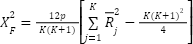
Each algorithm is evaluated on the following aspects: Convergence (best-so-far vs. iteration), Final solution quality (mean and standard deviation over independent runs), computational cost (wall clock time per run), scalability (quality as problem size increases), and robustness (dispersion of runs). The Friedman test of (23) ranks all the algorithms over all problems and tests the null hypothesis of no difference in performances, then the Wilcoxon signed-rank test is used to rank each pair of algorithms, based on the standard non-parametric procedure for comparing the performances of optimizers [26].
| 
| (23) |
Because the Friedman  statistic is conservative, the Iman–Davenport F statistic is also reported [26], and Kendall's coefficient of concordance,
 , serves as its effect size. Each Wilcoxon comparison is accompanied by the matched-pairs rank-biserial correlation
 , the winner on each problem is compared with the runner-up through Hedges' g, the Vargha–Delaney A12 statistic (the probability that a run of the winner ends lower than a run of the runner-up) and a paired Wilcoxon signed-rank test over the 20 seed-matched runs, and 95% confidence intervals of the mean are computed with the t distribution, or with the percentile bootstrap (10,000 resamples) where the t-interval would extend below the minimum of a non-negative objective. To decide whether a change of ranking between problem classes is statistically meaningful, the inversion statistic of (24) is used: the Spearman correlation
 between the optimizers' average ranks over the synthetic block and over the categorical domain block, with an exact permutation p-value computed over the set
 of all splits of the problems into blocks of the same sizes. An inversion is declared significant when < 0 and p < 0.05.
| 
| (24) |
EXPERIMENTAL SETUP
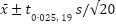
All experiments follow an identical protocol so that the comparison is fair. Each algorithm is run with a population of 30 individuals for 300 iterations on every problem, and each (algorithm, problem) pair is repeated over 20 independent runs with a fixed family of seeds shared across algorithms, so that comparisons are paired. Synthetic functions use dimension D = 30; the domain problems use their native dimensions (40 cloud tasks, 40 edge tasks, 50 IoT nodes, 30 6G users). Algorithm parameters follow common practice: PSO uses an inertia weight decaying linearly from 0.9 to 0.4 with cognitive and social coefficients of 1.49; GWO and WOA decay their control parameter from 2 to 0; DE uses the DE/rand/1/bin scheme with F = 0.5 and CR = 0.9; and SOA uses the cosine and linear schedules of (18), the exploration probability a/4, and secant-step clipping to ±0.5( ) as specified in Algorithm 2. The complete parameter settings of all six optimizers, with their sources, are listed in Table 2. The framework is implemented in Python (NumPy/SciPy) and all problem generators are seeded (seed = 2026) so that every instance, table and figure can be regenerated exactly. Alongside means and standard deviations, 95% confidence intervals of the mean are obtained as
 , and the significance protocol of Section 3.6 is applied without modification. Every optimizer evaluates the objective n times at initialization and n times per iteration, that is = 9,030 evaluations per run, which was verified by counting the objective calls of every optimizer on every problem; the peak memory allocated during a run, measured with Python's tracemalloc module, was between 24 kB and 128 kB. All experiments were run in a single process on a Linux virtual machine with an Intel Xeon processor at 2.80 GHz (2 vCPUs, 8 GB RAM), using Python 3.13.16, NumPy 2.5.3 and SciPy 1.18.1; the main experiment of 1,080 runs took 361 s of wall-clock time.
Table 2. Parameter settings of the six optimizers
Optimizer | Parameter | Value | Source |
All | Population size ; iterations ; independent runs | 30; 300; 20 | Identical budget |
All | Objective evaluations per run | = 9,030 | Identical budget |
All | Random seeds | master seed  = 2026; run seed s0 + | Paired comparisons |
All | Boundary handling | Clipping to  after every move | This study |
GA | Selection | Tournament, size k = 3 | [6] |
GA | Crossover | ,  = 0.5, probability  = 0.9 | [6] |
GA | Mutation | Gaussian, rate 0.1 per gene, standard deviation σ = 0.1() | [6] |
GA | Replacement | Generational with elitism: the best parent replaces the worst offspring (1 elite) | [6] |
PSO | Inertia weight w; coefficients  ,  ; velocity limit | Linear decrease 0.9 → 0.4; 1.49, 1.49; 0.2() | [7] |
GWO | Control parameter a | Linear decrease 2 → 0 | [8] |
WOA | Control parameter  ; spiral constant ; switch probability | Linear decrease 2 → 0; 1; 0.5 | [9] |
DE | Strategy; scale factor ; crossover rate | DE/rand/1/bin; 0.5; 0.9 | [10] |
SOA | Exploitation weight  ; amplitude a | Cosine and linear schedules, (18) | [16] |
SOA | Exploration probability; secant-step clip;  in (16) | a/4; ±0.5();  | [16], Algorithm 2 |
RESULTS AND DISCUSSION
Performance on Synthetic Functions
Table 3 reports the mean and standard deviation of the final objective on the five synthetic functions, and Figure 3 shows the corresponding convergence on a logarithmic scale. The exploitation-oriented swarm optimizers dominate this regime: WOA ranks first and GWO second on all five functions. WOA reaches the global minimum to within floating-point precision on Rastrigin, where 19 of its 20 runs end at exactly zero, on Ackley (5.06e-15) and on Griewank (5.55e-18), and approaches it on Sphere (7.61e-49); GWO follows at a larger but still negligible distance (3.71e-17 on Sphere and 1.66e-9 on Ackley), consistent with the rapid convergence for which both algorithms are known [8][9]. Rosenbrock is the exception: WOA has the lower mean (18.692 against 27.384) because 8 of its 20 runs entered the curved valley and ended between 0.49 and 10.44, whereas the other 12 stopped near 28.7, so its median run is slightly worse than that of GWO (28.69 against 27.12) and the difference is not significant Table 8.
Below the two leaders the ordering varies from function to function. SOA is third on Sphere, Rosenbrock and Griewank, with a Sphere mean (0.096) an order of magnitude below that of PSO (1.362), but it is fifth on the strongly multimodal Rastrigin function (158.004 ± 36.632) and last on Ackley (15.414 ± 8.116), where secant steps extrapolated from a single fitness difference towards the current best are repeatedly misled by the dense, regular local minima. DE/rand/1 does not converge to the incumbent best, but rather perturbs a random base vector, and hence has a slow convergence rate under the fixed budget with the Sphere mean of 36.231, which is spiked by four runs above 100, and the median run of 3.30. The real-coded GA is last on Sphere, Rosenbrock and Griewank, since the Gaussian mutation, which is one-tenth of the search range, is large compared to the neighbourhood of the optimum. Agreements between the five functions are good (Kendall's  = 0.81, p = 0.001), which is an important stability in the top of the synthetic ranking, which makes the reverse reported in the following subsection significant.
Table 3. Mean ± standard deviation over 20 runs of the final result on the synthetic functions (lower is better; = 30)
Problem | GA | PSO | GWO | WOA | DE | SOA |
Sphere | 473.704 ± 80.244 | 1.362 ± 1.444 | 3.71e-17 ± 5.84e-17 | 7.61e-49 ± 1.38e-48 | 36.231 ± 73.018 | 0.096 ± 0.050 |
Rastrigin | 119.305 ± 18.770 | 68.996 ± 17.112 | 17.883 ± 11.216 | 2.84e-15 ± 1.27e-14 | 192.991 ± 14.536 | 158.004 ± 36.632 |
Ackley | 6.142 ± 0.536 | 2.248 ± 0.715 | 1.66e-9 ± 1.84e-9 | 5.06e-15 ± 2.60e-15 | 2.058 ± 1.665 | 15.414 ± 8.116 |
Rosenbrock | 36281.2 ± 10498.0 | 345.950 ± 658.909 | 27.384 ± 0.968 | 18.692 ± 12.764 | 9630.9 ± 19197.7 | 219.715 ± 255.189 |
Griewank | 5.263 ± 0.722 | 0.548 ± 0.318 | 0.007 ± 0.012 | 5.55e-18 ± 2.48e-17 | 1.047 ± 0.779 | 0.450 ± 0.179 |
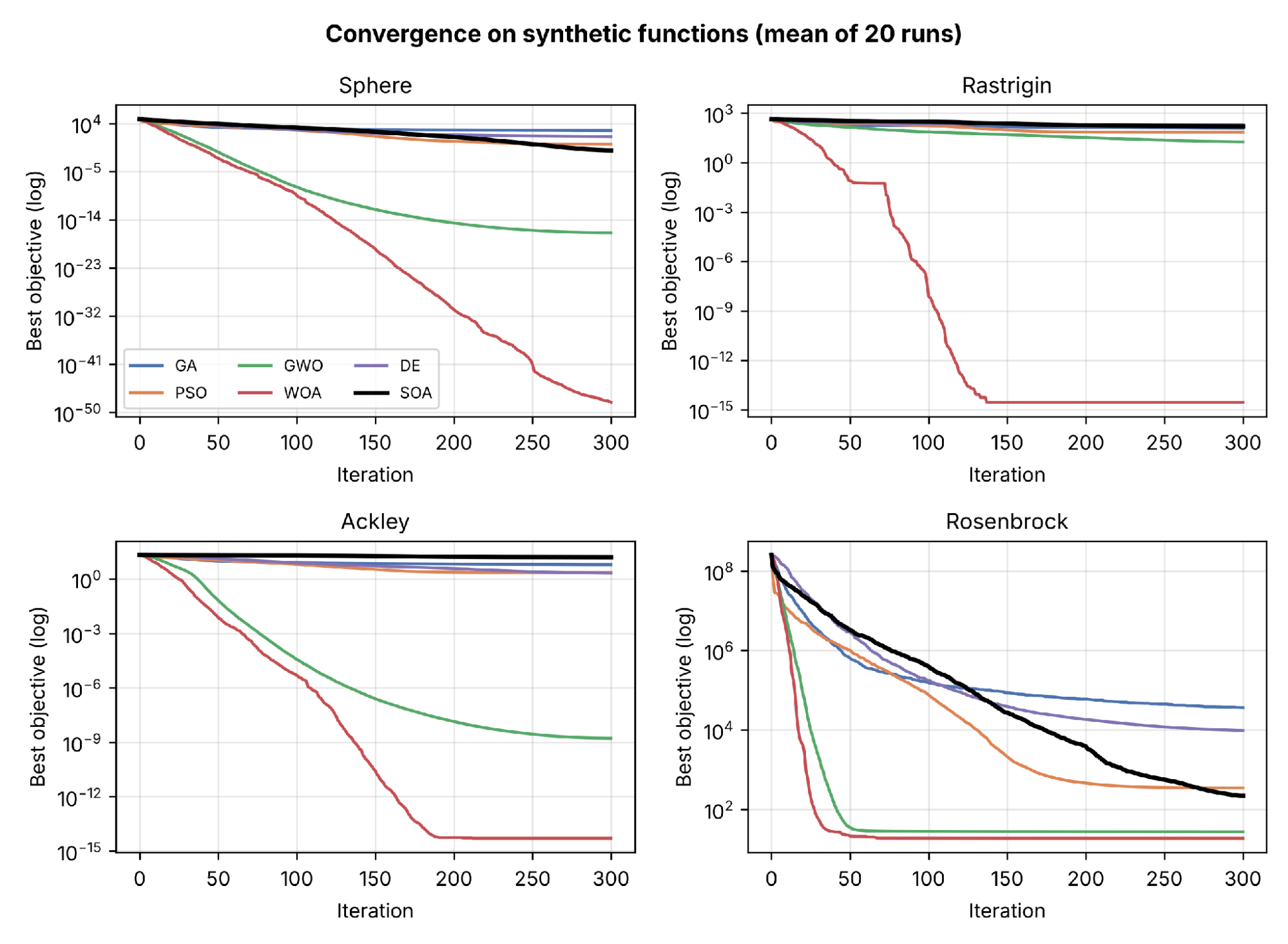
Figure 3. Convergence on four synthetic functions (mean best-so-far value over 20 runs, log scale). Under the fixed budget, WOA and GWO converge fastest, while the GA, DE and SOA remain far from the optimum after 300 iterations
Performance on Real-World Domain Problems
The picture changes on the domain models. Table 4 reports the mean and standard deviation on the four models and Figure 4 shows the corresponding convergence. The swarm optimizers that led the synthetic suite no longer lead: the GA obtains the best mean on all three models that become categorical after decoding, namely cloud scheduling (28.602 ± 0.518), edge offloading (164.105 ± 5.278) and IoT clustering (13.126 ± 0.100 mJ), whereas WOA, first on every synthetic function, is last on cloud scheduling and edge offloading and fourth on IoT clustering, and on the first two its convergence curve flattens well before the end of the budget Figure 4. The size of the GA's lead differs between the models. On edge offloading it is clear: the 95% interval of the GA, [161.635, 166.576], does not overlap that of the runner-up DE, [167.070, 173.886], and the paired comparison is significant Table 8. On cloud scheduling PSO is within 0.4% of the GA (28.720 ± 0.535), and on IoT clustering GWO and DE are within 0.2%; neither difference is significant, so on these two models the GA shares first place with its nearest competitors. What is robust on all three models is the gap between the GA and WOA (paired Wilcoxon p < 0.001, ≥ 0.975).
The 6G allocation model behaves differently from both blocks. All six optimizers lie within 0.073 of one another on an objective of magnitude 260, that is 0.028%, and the equal-power heuristic of Section 3.5 is within 0.022% of the best mean. PSO attains the nominal rank 1 (−260.2526 ± 9.19e-5), closely followed by GWO and DE, while WOA (−260.2082) and SOA (−260.1798) are fifth and sixth: WOA reaches the level of the equal split within the first ten iterations and improves little afterwards, and the SOA curve is still descending at = 300 Figure 4. This is the only domain model whose decision vector remains continuous after decoding, and its ranking is essentially uncorrelated with both the synthetic ranking  ) and the categorical one ( = 0.14): it neither preserves the synthetic order nor follows the reversal, and the differences on which its ranks rest are too small to matter in practice. The contrast between Table 3 and Table 4 on the three categorical models is the empirical core of this study and is tested in Section 5.4.
Table 4. The Mean ± standard deviation of the last objective obtained from 20 runs on the four real-world domain problems (lower is better; IoT clustering in mJ, 6G allocation as negative sum rate in Mbps plus penalty)
Problem | GA | PSO | GWO | WOA | DE | SOA |
Cloud-Scheduling | 28.602 ± 0.518 | 28.720 ± 0.535 | 30.397 ± 1.714 | 34.144 ± 2.619 | 31.341 ± 0.748 | 29.375 ± 0.999 |
Edge-Offloading | 164.105 ± 5.278 | 198.943 ± 14.468 | 177.645 ± 10.064 | 280.404 ± 29.134 | 170.478 ± 7.282 | 181.228 ± 12.495 |
IoT-Clustering | 13.126 ± 0.100 | 14.754 ± 1.276 | 13.142 ± 0.054 | 13.684 ± 0.285 | 13.152 ± 0.128 | 13.695 ± 0.456 |
6G-ResourceAlloc | −260.2355 ± 0.0039 | −260.2526 ± 9.19e-5 | −260.2523 ± 2.44e-4 | −260.2082 ± 0.0166 | −260.2519 ± 0.0019 | −260.1798 ± 0.0545 |
Table 5 gives these intervals for each algorithm–problem combination. Non-overlapping intervals are not due to run-to-run dispersion. This is true for the GA in the other comparisons with each optimizer in the other models, but not in the paired tests with PSO for cloud scheduling; it is also not true in the paired tests with GWO or DE for IoT clustering. The intervals of WOA and GWO are separated for the five synthetic functions, but for Rosenbrock the separation is due to the two sets of WOA runs as described in Section 5.1, and not a consistent advantage. For the functions WOA on Rastrigin and Griewank, nearly every run is unable to reach zero and the t-interval extends below the minimal value of the objective function, therefore the t-interval is not reported and the percentile-bootstrap interval is reported.
Table 5. 95% confidence intervals of the mean final objective (n = 20, t0.025,19 = 2.093). †Percentile-bootstrap interval (10,000 resamples), used where the t-interval would extend below the minimum of the objective
Problem | GA | PSO | GWO | WOA | DE | SOA |
Sphere | [436.148, 511.259] | [0.686, 2.037] | [9.84e-18, 6.45e-17] | [1.14e-49, 1.41e-48] | [2.057, 70.405] | [0.073, 0.119] |
Rastrigin | [110.521, 128.090] | [60.988, 77.005] | [12.634, 23.133] | [0, 8.53e-15]† | [186.188, 199.794] | [140.859, 175.148] |
Ackley | [5.891, 6.393] | [1.913, 2.582] | [8.00e-10, 2.52e-9] | [3.84e-15, 6.28e-15] | [1.278, 2.837] | [11.615, 19.212] |
Rosenbrock | [31367.9, 41194.4] | [37.571, 654.329] | [26.930, 27.837] | [12.718, 24.666] | [646.1, 18615.7] | [100.282, 339.147] |
Griewank | [4.925, 5.601] | [0.399, 0.697] | [0.001, 0.013] | [0, 1.67e-17]† | [0.682, 1.411] | [0.366, 0.534] |
Cloud-Scheduling | [28.360, 28.845] | [28.469, 28.970] | [29.595, 31.200] | [32.918, 35.370] | [30.991, 31.691] | [28.907, 29.843] |
Edge-Offloading | [161.635, 166.576] | [192.171, 205.714] | [172.935, 182.355] | [266.768, 294.039] | [167.070, 173.886] | [175.380, 187.076] |
IoT-Clustering | [13.079, 13.173] | [14.157, 15.351] | [13.117, 13.168] | [13.550, 13.817] | [13.092, 13.212] | [13.481, 13.909] |
6G-ResourceAlloc | [−260.2373, −260.2337] | [−260.2526, −260.2525] | [−260.2524, −260.2522] | [−260.2160, −260.2005] | [−260.2528, −260.2511] | [−260.2053, −260.1543] |
Figure 5 shows the distribution of the final objective over the 20 runs for two synthetic and two domain problems, complementing the means in Table 3 and Table 4. On Sphere and Rastrigin, WOA and GWO are both accurate and consistent, while the outlying runs of DE on Sphere explain why its mean (36.231) lies an order of magnitude above its median (3.30). On cloud scheduling the GA and PSO have the lowest medians and the narrowest boxes, so their lead reflects consistently better schedules rather than a few favorable runs, whereas WOA has both the highest median and the widest spread (30.30 to 38.31). On 6G allocation the medians of PSO, GWO and DE coincide within 10−3, the GA lies slightly above them, and WOA and SOA are visibly dispersed, SOA with two runs above −260.06, which is consistent with its convergence curve still descending at T = 300 Figure 4.
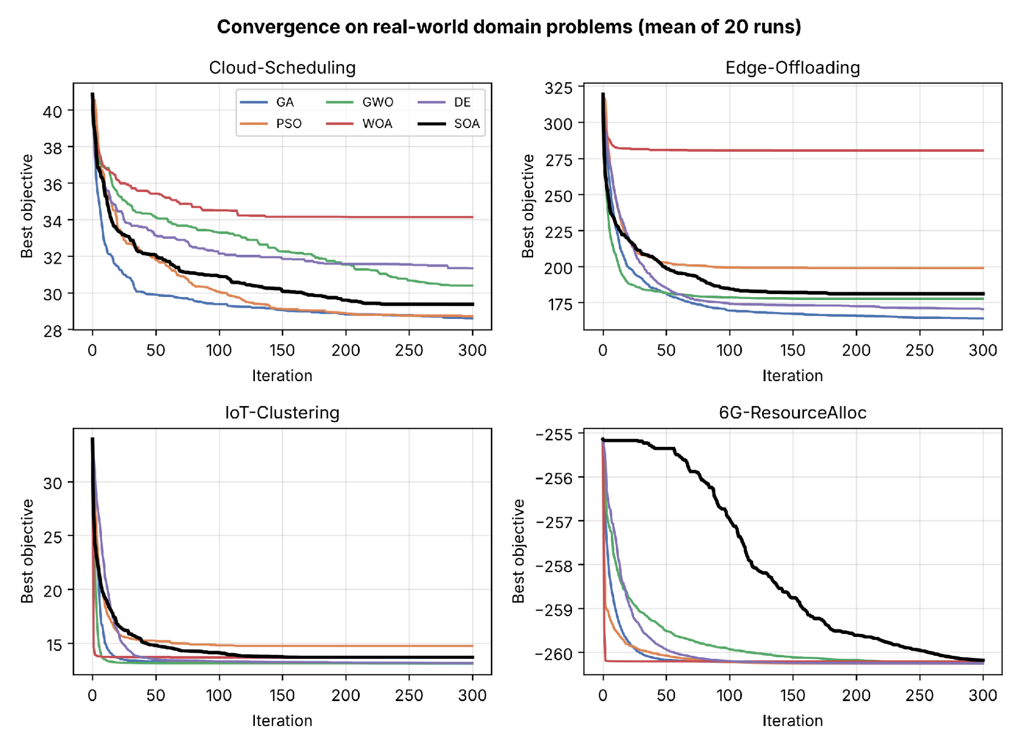
Figure 4. Convergence on the cloud, edge, IoT and 6G domain problems. The rankings are different from the synthetic case, with the GA leading on the three categorical models and WOA stagnating well before the end of the budget on cloud scheduling and edge offloading; on 6G all curves approach nearly the same value, SOA most slowly
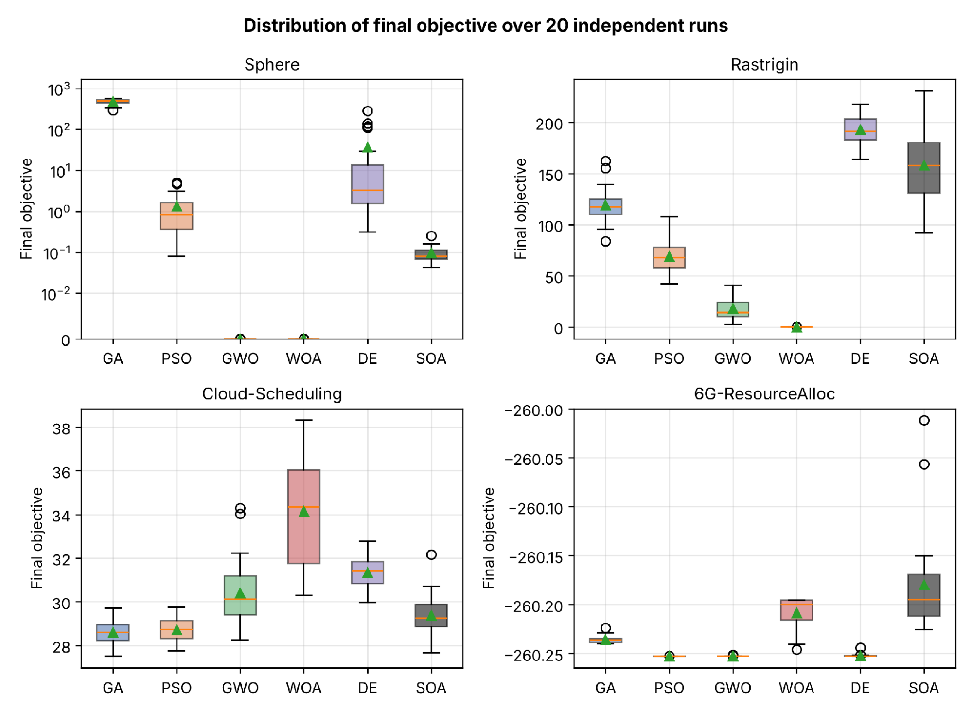
Figure 5. Central tendency and robustness to the run distribution of the final objective for 20 runs across two synthetic and two domain problems (box: interquartile range; line: median; triangle: mean; Sphere on a symmetric logarithmic scale)
Statistical Ranking and Significance
Aggregated over all nine problems, the average Friedman ranks Table 6 place GWO first (2.33), followed by WOA (2.89), PSO (3.67), the GA (3.78), DE (4.11) and SOA (4.22). The Friedman test does not reject the null hypothesis that the six optimizers are equivalent ( = 7.03,  = 0.218), the less conservative Iman–Davenport statistic gives the same conclusion ((5, 40) = 1.48, = 0.217), and the overall concordance is small (Kendall's = 0.16). This is not evidence that the optimizers perform alike: within the synthetic block the five functions agree strongly (W = 0.81, = 20.20, = 0.001), and within the categorical block the three models agree moderately ( = 0.62, p = 0.098). The pooled ranks are flat because the two blocks order the optimizers in nearly opposite ways, so that their ranks cancel when pooled; this is the inversion examined in Section 5.4, and it is why the per-block and per-problem analyses carry more information than the aggregate rank.
Consistently, the Nemenyi post-hoc critical difference for  = 6 algorithms on = 9 problems at = 0.05, CD =
 = 2.850 × 0.882 = 2.51, exceeds the largest gap in average rank, 1.89 between GWO and SOA, so no pair is separated by the post-hoc test Figure 6. The complete rank matrix is shown in Figure 7, where the domain dependence is directly visible: WOA and GWO dominate the synthetic rows, whereas the GA is first in the cloud, edge and IoT rows, and WOA falls to the bottom half of them.
The pairwise Wilcoxon tests in Table 7 compare SOA, the newest optimizer in the pool, with each of the other five across the nine problems. SOA ranks last on average (4.22), yet no comparison is significant after the Holm correction for five comparisons against a common control: the smallest unadjusted p-value, against GWO ( = 5, = 0.039,  = −0.78), becomes 0.195 after adjustment, and the remaining adjusted values equal 1.000. The effect sizes indicate a complex situation: SOA is significantly superior to GWO and slightly inferior to WOA ( = −0.78 and −0.47), while significantly inferior to PSO and DE, and only slightly superior to GA on five out of nine problems ( = −0.20, +0.38, and −0.07).
Table 6. Per-problem rank (1 = best), and average Friedman rank over all nine problems
Problem | GA | PSO | GWO | WOA | DE | SOA |
Sphere | 6 | 4 | 2 | 1 | 5 | 3 |
Rastrigin | 4 | 3 | 2 | 1 | 6 | 5 |
Ackley | 5 | 4 | 2 | 1 | 3 | 6 |
Rosenbrock | 6 | 4 | 2 | 1 | 5 | 3 |
Griewank | 6 | 4 | 2 | 1 | 5 | 3 |
Cloud-Scheduling | 1 | 2 | 4 | 6 | 5 | 3 |
Edge-Offloading | 1 | 5 | 3 | 6 | 2 | 4 |
IoT-Clustering | 1 | 6 | 2 | 4 | 3 | 5 |
6G-ResourceAlloc | 4 | 1 | 2 | 5 | 3 | 6 |
Average rank | 3.78 | 3.67 | 2.33 | 2.89 | 4.11 | 4.22 |
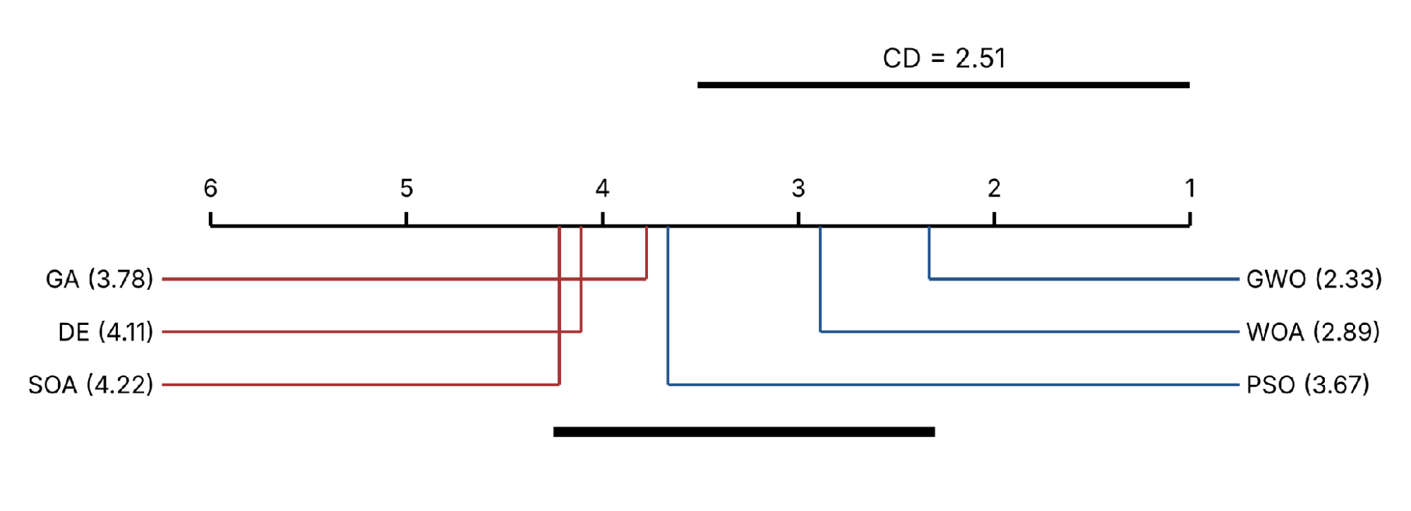
Figure 6. Critical-difference (Nemenyi) diagram of the average Friedman ranks over the nine problems (k = 6, N = 9, α = 0.05, CD = 2.51). The bar connects algorithms that are not significantly different; no pair is separated at the 5% level
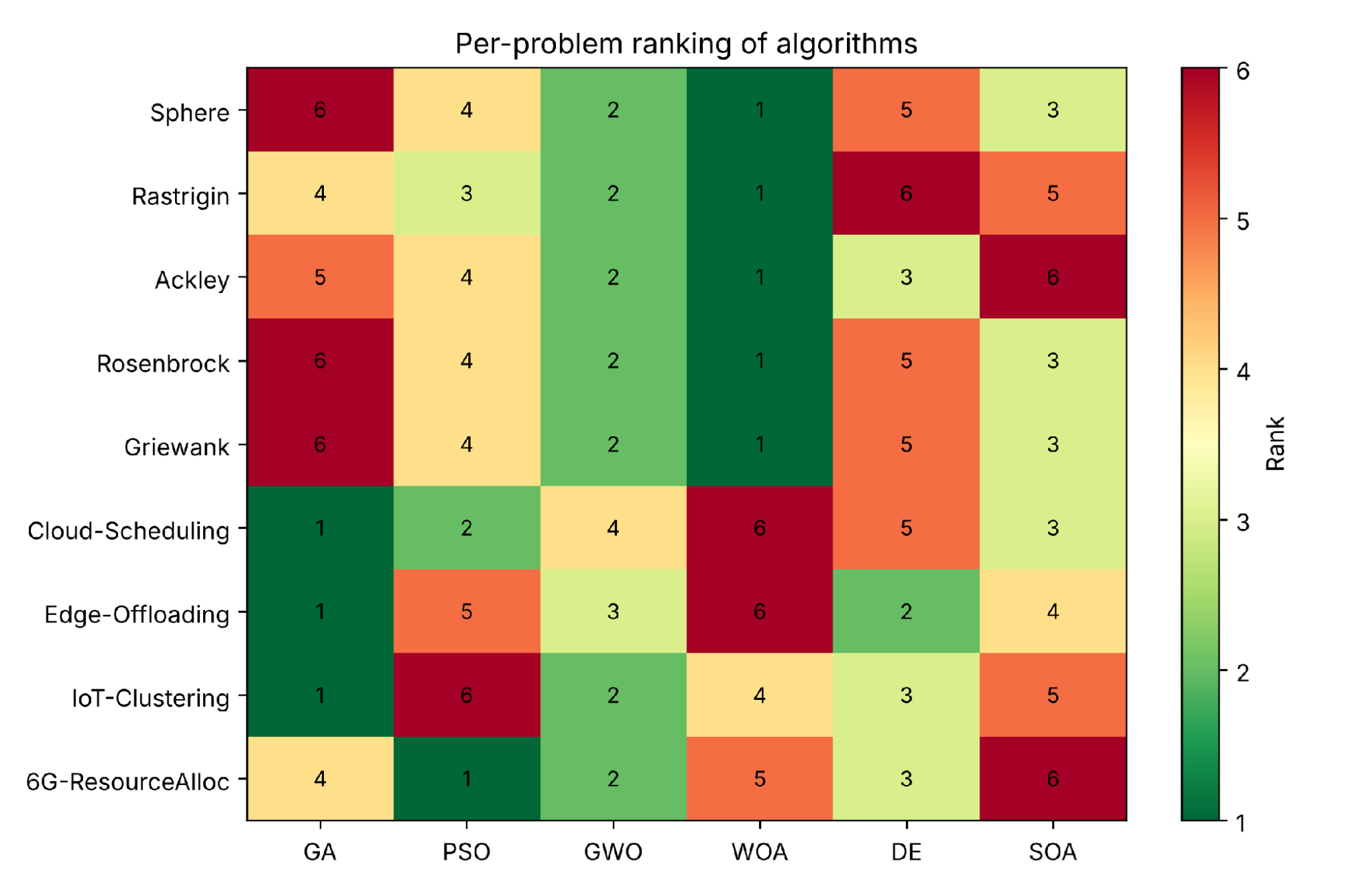
Figure 7. Per-problem ranking heatmap. The ranking inversion mentioned in Section 5.4 is what is seen in the synthetic rows and the domain rows
Table 7. Wilcoxon signed-rank comparison of SOA against each other algorithm across the nine problems (mean final objective per problem), with Holm-adjusted p-values and rank-biserial effect sizes (positive rrb favors SOA)
Comparison | W (W+ / W−) | Exact p | Holm p |
| Problems on which SOA is lower |
SOA vs. GA | 21 (24 / 21) | 0.910 | 1.000 | −0.07 | 3 of 9: Sphere, Rosenbrock, Griewank |
SOA vs. PSO | 18 (18 / 27) | 0.652 | 1.000 | +0.20 | 5 of 9: Sphere, Rosenbrock, Griewank, Edge-Offloading, IoT-Clustering |
SOA vs. GWO | 5 (40 / 5) | 0.039 | 0.195 | −0.78 | 1 of 9: Cloud-Scheduling |
SOA vs. WOA | 12 (33 / 12) | 0.250 | 1.000 | −0.47 | 2 of 9: Cloud-Scheduling, Edge-Offloading |
SOA vs. DE | 14 (14 / 31) | 0.359 | 1.000 | +0.38 | 5 of 9: Sphere, Rastrigin, Rosenbrock, Griewank, Cloud-Scheduling |
SOA is therefore a mid-pool newcomer whose average rank is depressed mainly by the multimodal Rastrigin and Ackley functions and by its slow convergence on the 6G model, rather than by uniform inferiority; equally, the evidence does not support any claim that SOA outperforms the established baselines, and none is made. The win counts in Figure 8 complete the picture: WOA achieves rank 1 on the five synthetic functions, the GA on the three categorical models, and PSO on the 6G model.
Effect sizes also separate differences that are statistically detectable from differences that matter in practice Table 8. On edge offloading the lead of the GA over DE is large in both senses: g = 0.98, A12 = 0.79, a mean cost 3.7% lower and a paired p < 0.001. On cloud scheduling and IoT clustering, by contrast, the lead of the GA over the runner-up is small (g = 0.22 and 0.20, A12 = 0.57 and 0.65) and not significant, so first place on those models is shared. On Sphere, Ackley and Griewank the lead of WOA over GWO is statistically clear (A12 ≥ 0.97, p < 0.001) but practically irrelevant, because both optimizers end within 0.01 of the optimum, whereas on Rastrigin it is both significant and substantial (17.88 on average), and on Rosenbrock it is not significant. On 6G the difference between PSO and GWO is significant (p < 0.001) yet amounts to about one part in a million of the objective, which shows why significance alone is not a sufficient basis for ranking claims.
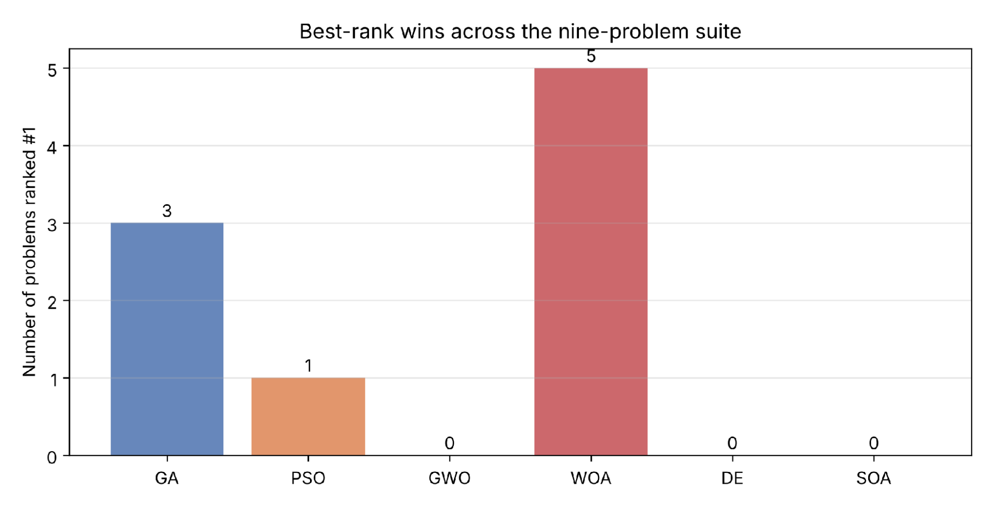
Figure 8. Number of problems on which each algorithm achieves rank 1
Table 8. Effect size of each per-problem winner (lowest mean) against the runner-up: Hedges' g and Vargha–Delaney from the 20 runs of each algorithm, and the p-value of the paired Wilcoxon signed-rank test over the seed-matched runs
Problem | Winner vs. runner-up | Mean difference | Hedges' g |
| Paired p | Practically meaningful |
Sphere | WOA vs. GWO | 3.71e-17 | 0.88 | 1.00 | <0.001 | No: both at numerical zero |
Rastrigin | WOA vs. GWO | 17.883 | 2.21 | 1.00 | <0.001 | Yes |
Ackley | WOA vs. GWO | 1.66e-9 | 1.25 | 1.00 | <0.001 | No: both at numerical zero |
Rosenbrock | WOA vs. GWO | 8.691 (31.7%) | 0.94 | 0.46 | 0.261 | No: median run of GWO is lower |
Griewank | WOA vs. GWO | 0.007 | 0.82 | 0.97 | <0.001 | No: both below 0.01 |
Cloud-Scheduling | GA vs. PSO | 0.117 (0.4%) | 0.22 | 0.57 | 0.522 | No: 0.4% difference |
Edge-Offloading | GA vs. DE | 6.373 (3.7%) | 0.98 | 0.79 | <0.001 | Yes |
IoT-Clustering | GA vs. GWO | 0.016 (0.1%) | 0.20 | 0.65 | 0.287 | No: 0.1% difference |
6G-ResourceAlloc | PSO vs. GWO | 2.49e-4 | 1.33 | 0.93 | <0.001 | No: about 10−6 of the objective |
The Ranking Inversion and Its Interpretation
The framework's principal finding is a ranking inversion between the synthetic functions and the categorically decoded domain models. WOA, first on all five synthetic functions, falls to rank 6 on cloud scheduling and edge offloading and to rank 4 on IoT clustering, and GWO, second on all five, falls to ranks 4, 3 and 2, while the GA, last on the synthetic block (average rank 5.4), is first on all three categorical models. The inversion is a feature of these three and not a law in general – it is stated here in this limited context intentionally – on the fourth domain problem, 6G power allocation, the landscape is almost flat, all six optimizers agree within 0.028%, ranking does not follow block, a blanket claim that the GA is the best optimizer on real-world problems would misrepresent the data. The behavior shown in the three categorical models is what the No-Free-Lunch theorem [22] permits, but it is seldom displayed in one controlled study; the two problem cultures are usually studied separately [20][21],[31].
The analysis in Section 3.2 suggests the following explanation. The spiral and encircling moves of WOA and the three-leader moves of GWO decrease with the distance to the current leaders and converge as the population becomes closer; the decoded cloud, edge, and IoT objectives are piecewise constant, and as the moves get shorter than a band, a more significant portion of the evaluations do not change the decoded solution (and thus the objective) (4). The property of the GA which prevents fine convergence is the most weak one—it is the same property that causes the GA to cross band boundaries in the case of the Gaussian mutation (whose standard deviation is fixed at one tenth of the range). This is because the structure of the decoded objective is what matters, not the term 'synthetic' or 'real-world' (but directly confirming this explanation needs an encoding ablation listed in Section 5.6.4). The real-world impact is immediate: An optimizer that seems to be best on one set of synthetically-generated data may be worse—just as bad as the optimizers it claimed to be better at—when deployed on a scheduling or offloading workload.
The inversion statistic of (24) is used to determine if this reversal is statistically significant. The average rank for each of the five synthetic functions is correlated with the average rank of the three categorical models and significance is tested exactly for all 56 splits of the 8 problems into blocks of 5 and 3. With the 6G model included in the domain block, the observed split is ρinv = −0.66 (Kendall τ = −0.60), which is the most extreme of all 56 (p = 0.018); with the nine problems included in the domain block, the observed split is ρinv = −0.60, and only 2 of the 126 splits of the nine problems are as extreme (p = 0.016). Within the blocks there is agreement for the synthetic functions (Kendall's W = 0.81, p = 0.001) and moderate for the categorical models (W = 0.62, p = 0.098): the GA is first and WOA is in the bottom half, while the middle of the ranking varies by model. The inversion is then a statistically significant reversal of the synthetic ordering at its extremes, and not a new synthetic ordering which is equally stable.
Computational Cost and Scalability
Deployability isn't just about the quality of the solution, it's about the cost of it. The wall-clock time per run averaged over all 9 problems is given in Table 9. The cheapest methods are PSO (0.179 s) followed by GWO (0.198 s) and WOA (0.258 s), while SOA (0.409 s) and the GA (0.428 s) are in the middle of the cost range, the first due to the secant-step computation and the second due to the application of clipping to each agent and the tournament selection/recombination of the offspring. DE is the most expensive method (0.532 s), since trial vectors are generated and selected one by one. The differences are a result of the overhead of the operators, as they make exactly 9,030 evaluations, regardless of the optimizer, and do not depend on the number of objective calls.
The spread between the fastest and the slowest optimizer is a factor of 3.0, which is small in absolute terms, since no algorithm exceeds 0.6 s per run at this scale; runtime alone therefore does not discriminate between the methods, and selection should be governed by the quality–cost trade-off. The absolute times depend on the implementation and the hardware of Section 4, and would change with compiled or fully vectorized code, whereas the quality results above do not depend on them.
Scalability is examined on the cloud-scheduling problem as the number of tasks grows from 20 to 100, with an instance generated with seed 2026 at each size and 10 runs per cell. As Table 10 and Figure 9 show, the GA has the lowest mean at four of the five sizes; at 60 tasks PSO is best (39.72 against 40.23 for the GA), and at 80 tasks SOA is within 0.1% of the GA. The GA, PSO and SOA remain within 4.1% of the best mean at every size, whereas WOA is the weakest optimizer at every size, 18–31% above the best, and GWO and DE lie between the two groups.
Two conclusions follow. First, the domain-dependent ranking reported in Section 5.2 is not an artifact of a single instance size, since the separation between the leading group and WOA persists across a fivefold increase in the number of tasks. Second, the differences within the leading group are small at every size (at most 4.1%) and the GA is overtaken once, in line with the non-significant difference between the GA and PSO in the main experiment Table 8, so the scalability results support the separation between the GA–PSO–SOA group and WOA rather than a strict ordering within the group. The relative gap between WOA and the best optimizer does not widen with the number of tasks (31.2% at 20 tasks and 21.6% at 100).
Table 9. Average wall-clock time per optimization run, aggregated over all problems
Algorithm | Mean time per run (s) |
GA | 0.428 |
PSO | 0.179 |
GWO | 0.198 |
WOA | 0.258 |
DE | 0.532 |
SOA | 0.409 |
Table 10. Scalability on cloud scheduling: mean objective as the number of tasks increases (10 runs per cell)
Tasks | GA | PSO | GWO | WOA | DE | SOA |
20 | 15.66 | 16.19 | 16.88 | 20.55 | 17.06 | 16.30 |
40 | 28.47 | 28.85 | 30.33 | 33.78 | 31.16 | 29.49 |
60 | 40.23 | 39.72 | 43.09 | 48.43 | 44.60 | 41.04 |
80 | 58.54 | 58.75 | 60.53 | 68.97 | 65.28 | 58.56 |
100 | 61.18 | 61.33 | 66.49 | 74.38 | 68.36 | 62.76 |
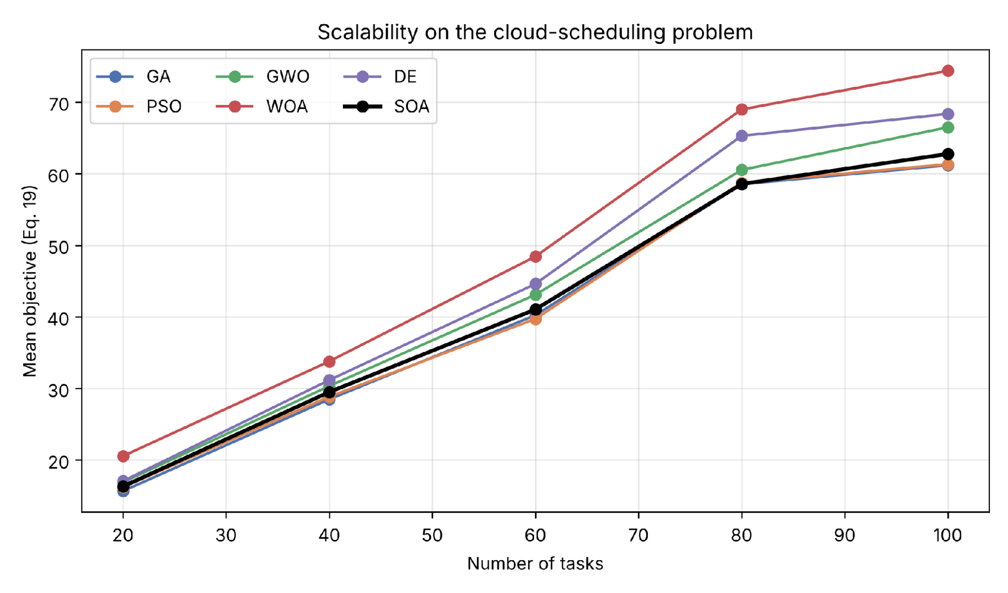
Figure 9. Scalability of the six optimizers on cloud scheduling as task count grows from 20 to 100
Discussion
Main Findings
Three findings emerge from Section 5.1 to Section 5.5. First, WOA and GWO lead on every synthetic function, but on the three models that become categorical after decoding the ordering reverses at its extremes: the GA, last on the synthetic block, has the best mean on cloud scheduling, edge offloading and IoT clustering, clearly on edge offloading and shared with its nearest competitors on the other two, while WOA falls to the lower half on all three. Second, this reversal is statistically significant under the criterion of (24) (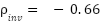 ,
 ), and it is strong enough to cancel the pooled Friedman ranking (
 ). Third, the reversal is conditional on the decoded structure: on the 6G model, whose decision vector stays continuous after decoding, neither ordering appears, all optimizers agree to within 0.028%, and a simple equal-power allocation is almost as good.
Comparison with Other Studies
The absolute objective values are not directly comparable with the values of bespoke studies on different instances of the HBF problems, however, the qualitative pattern is comparable and is also probably more informative. Recent domain studies are broadly consistent with this pattern, as summarized in Table 11: in cloud scheduling, GA–PSO hybrids remain standard baselines and standalone WOA has needed hybridization before becoming competitive [43][44]; leader-based GWO variants remain effective where the decision variables are continuous, as in joint power control for NOMA uplinks [53]; and swarm optimizers excel on smooth, continuous engineering benchmarks [8][9],[18]. A GWO-based framework that performs well in collaborative edge offloading [45] is not in conflict with these results: canonical GWO is third on the HBF edge model, behind the GA and DE, and the framework of [45] is designed for that problem rather than applied through band decoding.
The contribution of this paper is to reproduce all of these observations within one controlled, statistically tested framework and to expose the inversion that connects them—something the single-domain literature, by construction, cannot show. Relative to recent benchmarking reviews that catalogue test functions and call for more realistic, reproducible evaluation [20][21], the HBF is a concrete, executable answer rather than a recommendation, and relative to recent algorithm proposals that report superiority on a single suite [14]–[16], it provides the cross-domain context in which such claims should be read.
Relative to the general-purpose platforms summarized in Table 11, the distinction is one of coverage rather than of sophistication. COCO/BBOB [27] and IOHprofiler with its analysis module IOHanalyzer [28] provide considerably more mature performance-assessment machinery than HBF — runtime distributions, fixed-target and fixed-budget analyses, and large curated suites — but both remain within the synthetic problem class, and where IOHprofiler does cover discrete problems these form a separate pseudo-Boolean suite rather than application models sharing an interface with the continuous ones. The contribution of HBF is to place four communication–computing models behind the same interface and the same statistical protocol as the synthetic functions. Conversely, the domain studies reviewed in Section 2.2 model their applications in far greater detail than the four generators used here, but each evaluates a handful of algorithms on a single problem, which is precisely the configuration in which a ranking inversion cannot be detected. The results of Section 5.4 also give an empirical illustration of the concern raised by Kudela [31], that conclusions drawn from synthetic suites may fail to survive a change of problem class, and they point to the structure of the decoded objective as the likely mechanism.
Table 11. Comparison of HBF findings with recent domain studies
Study | Domain | Optimizers compared | Best reported | Relation to HBF |
Sandhu et al. [44] | Cloud task scheduling | Hybrid of tabu search, Bayesian classification and WOA vs. a GA–PSO hybrid and standalone WOA | Hybrid | Consistent: plain WOA needed hybridization; WOA ranks last (6th) on HBF cloud scheduling |
Karim et al. [43] | Cloud scheduling (makespan, utilization) | Dung-beetle-based scheduler vs. five schedulers, including a hybrid PSO–GA | Dung-beetle-based scheduler, at the highest run time | Consistent: problem-specific methods win; on HBF cloud scheduling a list-scheduling heuristic also beats all six generic optimizers |
Nujhat et al. [45] | Collaborative edge offloading | GWO-based framework vs. MGBD, iRAF and MOEA/D | GWO-based framework | Not in conflict: canonical GWO ranks 3rd of 6 on HBF edge offloading; the framework is problem-specific |
Sikkanan et al. [53] | NOMA uplink power control and user grouping | Multi-learning GWO vs. standard GWO and other algorithms | Multi-learning GWO | Partly consistent: GWO ranks 2nd on the continuous HBF 6G model, although all optimizers lie within 0.028% there |
Implications and explanation of findings
The band-crossing analysis of (3) to (4) is consistent with these findings: operators whose step lengths contract towards zero lose effectiveness when the objective is piecewise constant, whereas operators that keep a minimum step length, such as the fixed-scale Gaussian mutation of the GA, keep crossing band boundaries. Three implications follow. For researchers, the superiority of a new optimizer on a synthetic suite is evidence about smooth landscapes only; reporting results on both problem classes, with effect sizes and per-run raw data, would make such claims testable. The encoding is part of the algorithm: a practitioner should check an algorithm for a scheduling or offloading workload on a decoded version of the workload, and a continuous-encoding pipeline should favor operators with a minimum step length. Finally, the generic optimizers should be compared to a problem-specific constructive heuristic as this heuristic performed better than all six at the current budget on the cloud model.
Strengths and limitations
The advantages of the study are the paired design in which all the optimizers are passed instances, budgets and seeds; two problem classes under one statistical protocol; the reporting of effect size and confidence interval in addition to the significance test; and a fully specified, seeded implementation with code, seeds and raw results that can be regenerated, allowing all numbers to be recreated. It has the following drawbacks.
First, the domain models are realistic in structure, but are abstractions of simplified systems that in reality are multi-objective and dynamic; the objectives in the cloud and edge are aggregated into weighted sums, where the reported results are dependent on the weights and might be improved by true Pareto analysis. Second, the continuous encoding that makes the framework uniform also dulls the swarm optimizers on the discrete landscapes, so some of the observed inversion is due to the encoding as well as the algorithms, and native discrete operators would complement and help tease apart this effect.
Third, the comparison covers six optimizers under a fixed 300-iteration budget, and all six optimizers were implemented within the framework from their published descriptions rather than taken from reference code, so the rankings, in particular that of the recent SOA, should be read as indicative; a larger algorithm pool, longer budgets, and the authors' original implementations would sharpen the conclusions. None of these caveats affects the central, statistically supported finding—that rankings invert between the synthetic functions and the categorically decoded models—but each defines a clear avenue for the future work outlined in Section 6.
Fourth, the ranking inversion is established on three categorically decoded models, while the fourth domain problem remains continuous after decoding and does not show it; the finding must therefore not be generalized to all realistic problems, and a larger set of domain models, in particular discrete 6G formulations such as slice or subcarrier assignment, would be required to test whether the pattern holds where the 6G decision variables are themselves categorical. Fifth, pooled over nine problems, the Friedman and Nemenyi procedures do not separate the optimizers Section 5.3, so the average ranks carry no claim of overall superiority; the conclusions rest on the block-wise and per-problem analyses, and enlarging the problem library is the direct remedy. Sixth, the domain models do not separate every optimizer from simple baselines: on cloud scheduling a longest-task-first list-scheduling heuristic (27.85) is better than the mean of every optimizer, including the GA (28.60), at the budget of 9,030 evaluations, and on the 6G model equal power allocation is within 0.022% of the best mean. The rankings therefore compare generic optimizers with one another and do not show that they are the best available methods for these problems.
Seventh, several analyses requested for benchmarking studies are not part of the present protocol: a systematic sensitivity study of the optimizer parameters, an ablation of the encoding against alternative decoders, evaluation on the shifted and rotated CEC suites, a larger pool of recent adaptive optimizers, and instances drawn from public workload traces. The CEC suites would also test whether the lead of WOA and GWO depends on optima located at the center of the search space, a concern raised for several recent optimizers [31],[41]; it is consistent with this concern that Rosenbrock, the only synthetic function whose optimum is not at the origin, is also the only one on which WOA's lead over GWO is not significant. Each of these analyses is supported by the framework without changes to the problems or the statistics, and they are the first extensions listed in Section 6.
CONCLUSION AND FUTURE WORK
This paper introduced the Hybrid Benchmark Framework (HBF), a seeded evaluation engine that places synthetic test functions and models of the cloud, edge, IoT and 6G continuum behind a single continuous-encoding interface and a single statistical protocol. Its purpose is not to crown an optimizer but to test whether an optimizer's advantage survives a change of problem class.
Three findings emerge. First, the ranking obtained on smooth synthetic functions did not transfer to the models that become categorical after decoding: WOA, which led the synthetic suite, fell to the lower half of the table on cloud scheduling, edge offloading and IoT clustering, where the GA, last on the synthetic functions, had the best mean. Second, it is not a spur-of-the-moment change in ranking, because no other division of the eight problems shows a worse negative rank correlation, and is sufficiently strong to offset the ranking when problems are combined. Third, the reversal is dependent on the decoded structure, with no reversal seen on the 6G model, on which the decision vector remains continuous after decoding, and all six optimizers performing almost identically.
The theoretical contribution is an operational form of the No-Free-Lunch theorem for decoded problems: the band-crossing analysis links the step-length dynamics of an operator to its effectiveness on piecewise-constant objectives, and so predicts when an inversion should be expected. The practical contribution is a reusable, seeded instrument. Researchers can add an optimizer or a problem without touching the rest of the pipeline and obtain directly comparable, statistically qualified results, and practitioners can check a candidate optimizer on a decoded model of their own workload, and against a constructive heuristic, before deployment. Reporting results on both problem classes, with effect sizes and per-run raw data, could complement synthetic-only suites such as CEC and BBOB as a standard for evaluating new metaheuristics.
The conclusions are bounded by four simplified single-objective domain models, six optimizers, a fixed evaluation budget and one encoding family. Future work will (i) add a parameter-sensitivity study and an encoding ablation with alternative decoders and native discrete operators, to separate encoding effects from algorithmic ones; (ii) extend the synthetic block with the shifted and rotated CEC suites and enlarge the optimizer pool with recent adaptive algorithms run from their reference implementations; (iii) add multi-objective and dynamic variants of the domain models, replace synthetic instances with public workload traces and industrial datasets, and include problem-specific heuristics and larger budgets as reference points; and (iv) extend the 6G model to categorical decisions such as slice and subcarrier assignment, to test whether the inversion appears there as well.
DECLARATION
Acknowledgements
The authors would like to express their sincere gratitude to Sohar University, Al-Kitab University, University of Information Technology and Communication, Al-Bayan University, University of Al-Ameed, and Northern Technical University for their support and contributions to this research.
REFERENCES
- A. M. Rahmani, A. Haider, P. Khoshvaght, F. S. Gharehchopogh, K. Moghaddasi, S. Rajabi, and M. Hosseinzadeh, “Optimizing task offloading with metaheuristic algorithms across cloud, fog, and edge computing networks: A comprehensive survey and state-of-the-art schemes,” Sustainable Computing: Informatics and Systems, vol. 45, p. 101080, 2025, https://doi.org/10.1016/j.suscom.2024.101080.
- C. Sharanya, M. P. Lakshmi, P. S. Velumani, S. Perumalla, S. Lakshmanaprakash, M. T. Jagtap, A. Choudhary, and P. Ramesh, “Network slicing concurrent resource allocation for improving service response of 6G network using a novel cycle-consistent spatial frequency self-attention network with Tasmanian devil optimization,” Int. J. Commun. Syst., vol. 38, no. 12, p. e70156, 2025, https://doi.org/10.1002/dac.70156.
- X. Ni, Z. Dong, and X. Rong, “Innovative application of 6G network slicing driven by artificial intelligence in the Internet of Vehicles,” Int. J. Netw. Manage., vol. 35, no. 2, p. e70004, 2025, https://doi.org/10.1002/nem.70004.
- A. Satouf, A. Hamidoğlu, Ö. M. Gül, A. Kuusik, L. Durak Ata, and S. Kadry, “Metaheuristic-based task scheduling for latency-sensitive IoT applications in edge computing,” Cluster Comput., vol. 28, no. 2, p. 143, 2025, https://doi.org/10.1007/s10586-024-04878-6.
- A. A. Abba Ari, F. Samafou, A. N. Njoya, A. C. Djedouboum, M. Aboubakar, and A. Mohamadou, “IoT-5G and B5G/6G resource allocation and network slicing orchestration using learning algorithms,” IET Netw., vol. 14, no. 1, p. e70002, 2025, https://doi.org/10.1049/ntw2.70002.
- S. Katoch, S. S. Chauhan, and V. Kumar, “A review on genetic algorithm: Past, present, and future,” Multimed. Tools Appl., vol. 80, no. 5, pp. 8091–8126, 2021, https://doi.org/10.1007/s11042-020-10139-6.
- J. Kennedy and R. Eberhart, “Particle swarm optimization,” in Proc. ICNN'95 – Int. Conf. Neural Networks, vol. 4, pp. 1942–1948, 1995, https://doi.org/10.1109/ICNN.1995.488968.
- S. Mirjalili, S. M. Mirjalili, and A. Lewis, “Grey wolf optimizer,” Adv. Eng. Softw., vol. 69, pp. 46–61, 2014, https://doi.org/10.1016/j.advengsoft.2013.12.007.
- S. Mirjalili and A. Lewis, “The whale optimization algorithm,” Adv. Eng. Softw., vol. 95, pp. 51–67, 2016, https://doi.org/10.1016/j.advengsoft.2016.01.008.
- R. Storn and K. Price, “Differential evolution – A simple and efficient heuristic for global optimization over continuous spaces,” J. Global Optim., vol. 11, no. 4, pp. 341–359, 1997, https://doi.org/10.1023/A:1008202821328.
- M. Dehghani, Z. Montazeri, E. Trojovská, and P. Trojovský, “Coati optimization algorithm: A new bio-inspired metaheuristic algorithm for solving optimization problems,” Knowledge-Based Syst., vol. 259, p. 110011, 2023, https://doi.org/10.1016/j.knosys.2022.110011.
- S. Zhao, T. Zhang, S. Ma, and M. Chen, “Dandelion optimizer: A nature-inspired metaheuristic algorithm for engineering applications,” Eng. Appl. Artif. Intell., vol. 114, p. 105075, 2022, https://doi.org/10.1016/j.engappai.2022.105075.
- B. Abdollahzadeh, F. S. Gharehchopogh, N. Khodadadi, and S. Mirjalili, “Mountain gazelle optimizer: A new nature-inspired metaheuristic algorithm for global optimization problems,” Adv. Eng. Softw., vol. 174, p. 103282, 2022, https://doi.org/10.1016/j.advengsoft.2022.103282.
- M. H. Amiri, N. Mehrabi Hashjin, M. Montazeri, S. Mirjalili, and N. Khodadadi, “Hippopotamus optimization algorithm: A novel nature-inspired optimization algorithm,” Sci. Rep., vol. 14, no. 1, p. 5032, 2024, https://doi.org/10.1038/s41598-024-54910-3.
- W. Zhao, L. Wang, Z. Zhang, H. Fan, J. Zhang, S. Mirjalili, N. Khodadadi, and Q. Cao, “Electric eel foraging optimization: A new bio-inspired optimizer for engineering applications,” Expert Syst. Appl., vol. 238, p. 122200, 2024, https://doi.org/10.1016/j.eswa.2023.122200.
- M. Q. Ibrahim, M. Qaraad, N. K. Hussein, M. A. Farag, and D. Guinovart, “Secant optimization algorithm for efficient global optimization,” Sci. Rep., vol. 16, no. 1, p. 6659, 2026, https://doi.org/10.1038/s41598-026-36691-z.
- T. Ivanovski, M. Brkić Bakarić, and M. Matetić, “Recent advances in metaheuristic algorithms,” Algorithms, vol. 19, no. 1, p. 19, 2026, https://doi.org/10.3390/a19010019.
- W. F. Mbasso, A. Harrison, Z. Liu, Z. Mamadiyarov, S. F. Al-Gahtani, and Z. M. S. Elbarbary, “How do metaheuristics exploit? A particle-level behavioral study across the CEC 2025 benchmark functions,” Evolutionary Intelligence, vol. 19, no. 3, p. 77, 2026, https://doi.org/10.1007/s12065-026-01190-7.
- K. Rajwar, K. Deep, and S. Das, “An exhaustive review of the metaheuristic algorithms for search and optimization: Taxonomy, applications, and open challenges,” Artif. Intell. Rev., vol. 56, no. 11, pp. 13187–13257, 2023, https://doi.org/10.1007/s10462-023-10470-y.
- A. P. Piotrowski, J. J. Napiorkowski, and A. E. Piotrowska, “Choice of benchmark optimization problems does matter,” Swarm Evolutionary Comput., vol. 83, p. 101378, 2023, https://doi.org/10.1016/j.swevo.2023.101378.
- M. Z. Naser, M. K. Al-Bashiti, A. Teymori Gharah Tapeh, A. Naser, V. Kodur, R. Hawileh, J. Abdalla, N. Khodadadi, A. H. Gandomi, and A. Dadras Eslamlou, “A review of benchmark and test functions for global optimization algorithms and metaheuristics,” WIREs Comput. Stat., vol. 17, no. 2, p. e70028, 2025, https://doi.org/10.1002/wics.70028.
- D. H. Wolpert and W. G. Macready, “No free lunch theorems for optimization,” IEEE Trans. Evol. Comput., vol. 1, no. 1, pp. 67–82, 1997, https://doi.org/10.1109/4235.585893.
- H. Mikram and S. El Kafhali, “Optimizing workflow scheduling for efficient resource utilization in scalable cloud computing data centers,” Simulation, vol. 101, no. 11, pp. 1133–1151, 2025, https://doi.org/10.1177/00375497251356490.
- A. LaTorre, D. Molina, E. Osaba, J. Poyatos, J. Del Ser, and F. Herrera, “A prescription of methodological guidelines for comparing bio-inspired optimization algorithms,” Swarm Evolutionary Comput., vol. 67, p. 100973, 2021, https://doi.org/10.1016/j.swevo.2021.100973.
- E. Osaba, E. Villar-Rodriguez, J. Del Ser, A. J. Nebro, D. Molina, A. LaTorre, P. N. Suganthan, C. A. Coello Coello, and F. Herrera, “A tutorial on the design, experimentation and application of metaheuristic algorithms to real-world optimization problems,” Swarm Evolutionary Comput., vol. 64, p. 100888, 2021, https://doi.org/10.1016/j.swevo.2021.100888.
- J. Derrac, S. García, D. Molina, and F. Herrera, “A practical tutorial on the use of nonparametric statistical tests as a methodology for comparing evolutionary and swarm intelligence algorithms,” Swarm Evolutionary Comput., vol. 1, no. 1, pp. 3–18, 2011, https://doi.org/10.1016/j.swevo.2011.02.002.
- N. Hansen, A. Auger, R. Ros, O. Mersmann, T. Tušar, and D. Brockhoff, “COCO: A platform for comparing continuous optimizers in a black-box setting,” Optimization Methods Software, vol. 36, no. 1, pp. 114–144, 2021, https://doi.org/10.1080/10556788.2020.1808977.
- H. Wang, D. Vermetten, F. Ye, C. Doerr, and T. Bäck, “IOHanalyzer: Detailed performance analyses for iterative optimization heuristics,” ACM Trans. Evol. Learn. Optim., vol. 2, no. 1, pp. 1–29, 2022, https://doi.org/10.1145/3510426.
- N. Van Thieu and S. Mirjalili, “MEALPY: An open-source library for latest meta-heuristic algorithms in Python,” J. Syst. Archit., vol. 139, p. 102871, 2023, https://doi.org/10.1016/j.sysarc.2023.102871.
- B. Huang, R. Cheng, Z. Li, Y. Jin, and K. C. Tan, “EvoX: A distributed GPU-accelerated framework for scalable evolutionary computation,” IEEE Trans. Evol. Comput., vol. 29, no. 5, pp. 1649–1662, 2025, https://doi.org/10.1109/TEVC.2024.3388550.
- J. Kudela, “A critical problem in benchmarking and analysis of evolutionary computation methods,” Nat. Mach. Intell., vol. 4, no. 12, pp. 1238–1245, 2022, https://doi.org/10.1038/s42256-022-00579-0.
- F. A. Hashim, E. H. Houssein, K. Hussain, M. S. Mabrouk, and W. Al-Atabany, “Honey badger algorithm: New metaheuristic algorithm for solving optimization problems,” Mathematics and Computers in Simulation, vol. 192, pp. 84–110, 2022, https://doi.org/10.1016/j.matcom.2021.08.013.
- F. A. Hashim and A. G. Hussien, “Snake optimizer: A novel meta-heuristic optimization algorithm,” Knowledge-Based Syst., vol. 242, p. 108320, 2022, https://doi.org/10.1016/j.knosys.2022.108320.
- L. Abualigah, M. Abd Elaziz, P. Sumari, Z. W. Geem, and A. H. Gandomi, “Reptile search algorithm (RSA): A nature-inspired meta-heuristic optimizer,” Expert Syst. Appl., vol. 191, p. 116158, 2022, https://doi.org/10.1016/j.eswa.2021.116158.
- J. O. Agushaka, A. E. Ezugwu, and L. Abualigah, “Dwarf mongoose optimization algorithm,” Comput. Methods Appl. Mech. Eng., vol. 391, p. 114570, 2022, https://doi.org/10.1016/j.cma.2022.114570.
- H. Su, D. Zhao, A. A. Heidari, L. Liu, X. Zhang, M. Mafarja, and H. Chen, “RIME: A physics-based optimization,” Neurocomputing, vol. 532, pp. 183–214, 2023, https://doi.org/10.1016/j.neucom.2023.02.010.
- M. Abdel-Basset, R. Mohamed, and M. Abouhawwash, “Crested porcupine optimizer: A new nature-inspired metaheuristic,” Knowledge-Based Syst., vol. 284, p. 111257, 2024, https://doi.org/10.1016/j.knosys.2023.111257.
- M. Hubálovská, Š. Hubálovský, and P. Trojovský, “Botox optimization algorithm: A new human-based metaheuristic algorithm for solving optimization problems,” Biomimetics, vol. 9, no. 3, p. 137, 2024, https://doi.org/10.3390/biomimetics9030137.
- M. Hubalovska and S. Major, “A new human-based metaheuristic algorithm for solving optimization problems based on technical and vocational education and training,” Biomimetics, vol. 8, no. 6, p. 508, 2023, https://doi.org/10.3390/biomimetics8060508.
- I. Ahmadianfar, A. A. Heidari, S. Noshadian, H. Chen, and A. H. Gandomi, “INFO: An efficient optimization algorithm based on weighted mean of vectors,” Expert Syst. Appl., vol. 195, p. 116516, 2022, https://doi.org/10.1016/j.eswa.2022.116516.
- C. L. Camacho-Villalón, M. Dorigo, and T. Stützle, “Exposing the grey wolf, moth-flame, whale, firefly, bat, and antlion algorithms: Six misleading optimization techniques inspired by bestial metaphors,” Int. Trans. Oper. Res., vol. 30, no. 6, pp. 2945–2971, 2023, https://doi.org/10.1111/itor.13176.
- C. Aranha, C. L. Camacho Villalón, F. Campelo, M. Dorigo, R. Ruiz, M. Sevaux, K. Sörensen, and T. Stützle, “Metaphor-based metaheuristics, a call for action: The elephant in the room,” Swarm Intell., vol. 16, no. 1, pp. 1–6, 2022, https://doi.org/10.1007/s11721-021-00202-9.
- F. K. Karim, S. Ghorashi, S. Alkhalaf, S. H. A. Hamza, A. Ben Ishak, and S. Abdel-Khalek, “Optimizing makespan and resource utilization in cloud computing environment via evolutionary scheduling approach,” PLOS ONE, vol. 19, no. 11, p. e0311814, 2024, https://doi.org/10.1371/journal.pone.0311814.
- R. Sandhu, M. Faiz, H. Kaur, A. Srivastava, and V. Narayan, “Enhancement in performance of cloud computing task scheduling using optimization strategies,” Cluster Comput., vol. 27, no. 5, pp. 6265–6288, 2024, https://doi.org/10.1007/s10586-023-04254-w.
- N. Nujhat, F. H. Shanta, S. Sarker, P. Roy, M. A. Razzaque, M. Mamun-Or-Rashid, M. M. Hassan, and G. Fortino, “Task offloading exploiting grey wolf optimization in collaborative edge computing,” J. Cloud Comput., vol. 13, no. 1, p. 23, 2024, https://doi.org/10.1186/s13677-023-00570-z.
- C. Kurangi, K. K. Paidipati, A. S. K. Reddy, J. Uthayakumar, G. Kadiravan, and S. Parveen, “Metaheuristic optimization-based clustering with routing protocol in wireless sensor networks,” Int. J. Commun. Syst., vol. 37, no. 16, p. e5914, 2024, https://doi.org/10.1002/dac.5914.
- R. Priyadarshi, “Energy-efficient routing in wireless sensor networks: A meta-heuristic and artificial intelligence-based approach: A comprehensive review,” Arch. Comput. Methods Eng., vol. 31, no. 4, pp. 2109–2137, 2024, https://doi.org/10.1007/s11831-023-10039-6.
- M. M. Shwaysh, A.-S. T. Hussain, S. Q. Salih, T. A. Almulaisi, A. D. Radhi, H. S. Majdi, and H. Desa, “Adaptive hybrid information gain and autoencoder-based feature selection with ensemble recurrent extreme learning machine for enhanced network intrusion detection systems,” J. Network Syst. Manage., vol. 34, no. 1, p. 11, 2025, https://doi.org/10.1007/s10922-025-09976-3.
- F. H. Taha, S. H. Hussein, M. T. Yaseen, H. A. Fadhil, S. A. Assi, H. Desa, A. I. Imran, A. D. Radhi, and T. Almulaisi, “Investigation and design of high efficiency quadrature power amplifier for 5G applications,” Int. J. Robot. Control Syst., vol. 5, no. 2, pp. 1481–1497, 2025, https://doi.org/10.31763/ijrcs.v5i2.1881.
- F. N. Hasoon, H. A. Fadhil, A.-S. T. Hussain, H. A. Kazem, and T. Almulaisi, “Development of new hybrid optical CDMA COARSE radio over fiber for 5G capacity improvement,” Int. J. Electron. Commun. Eng., vol. 13, no. 4, pp. 233–238, 2026, https://doi.org/10.14445/23488549/ijece-v13i4p119.
- S. A. Ahmed, M. R. B. Agha, Z. A. Abbood, A. H. Salih, M. A. Arif, A. D. Sallibi, A. M. Hussein, S. K. Mukhlif, and T. Almulaisi, “Anomaly detection in renewable energy SCADA systems using explainable AI techniques,” in 2026 2nd Int. Symp. AI-Driven Engineering Systems (ISADES), pp. 1–6, 2026, https://doi.org/10.1109/isades69945.2026.11608103.
- M. U. F. Qaisar, W. Yuan, O. Günlü, T. Riihonen, Y. Cui, L. Zhang, N. Gonzalez-Prelcic, M. Di Renzo, and Z. Han, “The role of ISAC in 6G networks: Enabling next-generation wireless systems,” IEEE Trans. Netw. Sci. Eng., vol. 13, pp. 7825–7861, 2026, https://doi.org/10.1109/TNSE.2026.3666665.
- S. Sikkanan, C. Kumar, P. Manoharan, and S. Ravichandran, “Exploring the potential of 5G uplink communication: Synergistic integration of joint power control, user grouping, and multi-learning grey wolf optimizer,” Sci. Rep., vol. 14, no. 1, p. 21406, 2024, https://doi.org/10.1038/s41598-024-71751-2.
- M. Becerra-Rozas, J. Lemus-Romani, F. Cisternas-Caneo, B. Crawford, R. Soto, G. Astorga, C. Castro, and J. García, “Continuous metaheuristics for binary optimization problems: An updated systematic literature review,” Mathematics, vol. 11, no. 1, p. 129, 2023, https://doi.org/10.3390/math11010129.
- J. Lemus-Romani, B. Crawford, F. Cisternas-Caneo, R. Soto, and M. Becerra-Rozas, “Binarization of metaheuristics: Is the transfer function really important?” Biomimetics, vol. 8, no. 5, p. 400, 2023, https://doi.org/10.3390/biomimetics8050400.
Hilal A. Fadhil (A Hybrid Benchmark Framework for Metaheuristic Optimization across Cloud, Edge, Internet-of-Things, and Sixth-Generation Communication Networks)