ISSN: 2685-9572 Buletin Ilmiah Sarjana Teknik Elektro
Vol. 8, No. 5, October 2026, pp. 1324-1345
A Comparative Study of Three Multi-Objective Formulations for NSGA-II-Based Multi-Robot Path Planning
Ariadie Chandra Nugraha 1,2, Oyas Wahyunggoro 1, Adha Imam Cahyadi 1
1 Department of Electrical Engineering and Information Technology, Universitas Gadjah Mada, Yogyakarta, Indonesia
2 Department of Electrical Engineering Education, Universitas Negeri Yogyakarta, Yogyakarta, Indonesia
ARTICLE INFORMATION |
| ABSTRACT |
Article History: Received 26 May 2026 Revised 27 June 2026 Accepted 15 September 2026 |
| 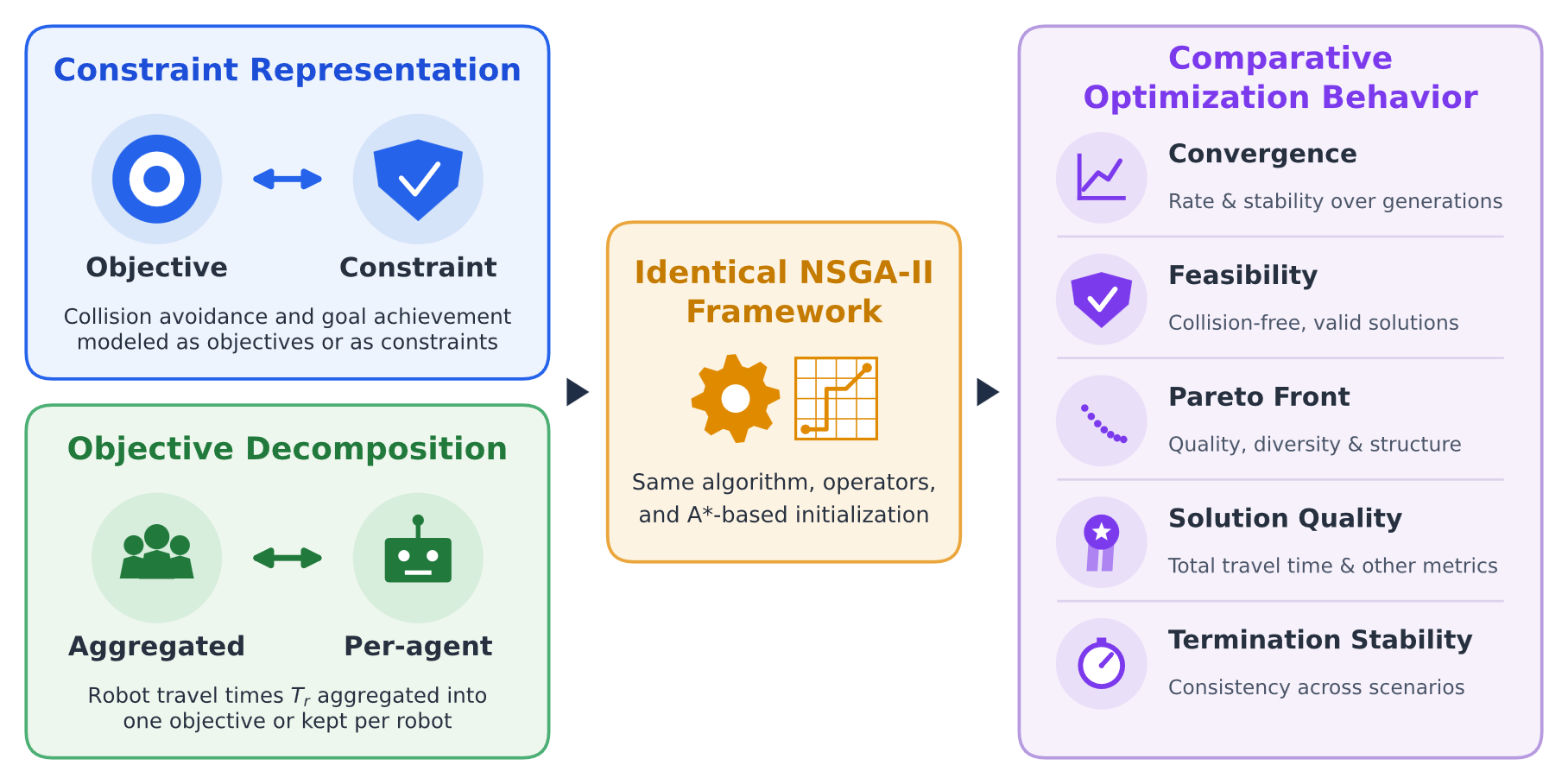
Existing works utilizing NSGA-II in multi-robot path planning have been primarily concerned with problem formulations where the aggregation of robot objectives, individuality of the objectives defined per each robot, and modeling of the collision avoidance through constraints and optimization objectives differ. The research contribution is systematic comparative analysis of three multi-objective optimization problem formulations within the same NSGA-II framework: (i) an aggregated objective formulation without constraints; (ii) a per-agent objective formulation with constraints; and (iii) a per-agent objective formulation without constraints. Initial population of NSGA-II are initialized using A* algorithm, while the formulations are tested on twelve scenarios comprising two to five robots for three 25 × 25 environments. Ten independent experiments are run for each scenario, and the non-parametric statistical tests are used. Aggregated and per-agent formulations with constraints maintain full feasibility for all scenarios and provide statistically equal results on the total travel time of up to four robots. On the other hand, the per-agent formulation without constraints loses feasibility and demonstrates highly inferior results for three or more robots. Front quality measures (hypervolume and inverted generational distance) calculated in a common objective space prove this and demonstrate the loss of diversity of the latter formulation in scenarios with five robots. The per-agent formulation with constraints is preferable: it matches the aggregated formulation in solution quality while exposing per-robot travel-time trade-offs and a clear Pareto front. This demonstrates the importance of problem formulation in affecting the convergence and termination behavior of NSGA-II. |
Keywords: Multi-Robot Path Planning; NSGA-II; Multi-Objective Optimization; Problem Formulation; Pareto Front; Collision Avoidance |
Corresponding Author: Oyas Wahyunggoro, Department of Electrical Engineering and Information Technology, Universitas Gadjah Mada, Yogyakarta, Indonesia
Email: oyas@ugm.ac.id |
This work is open access under a Creative Commons Attribution-Share Alike 4.0 
|
Document Citation: A. C. Nugraha, O. Wahyunggoro, and A. I. Cahyadi, “A Comparative Study of Three Multi-Objective Formulations for NSGA-II-Based Multi-Robot Path Planning,” Buletin Ilmiah Sarjana Teknik Elektro, vol. 8, no. 5, pp. 1324-1345, 2026, DOI: 10.12928/biste.v8i5.16915. |
Introduction
The goal of multi-robot path planning (MRPP) is to find trajectories along which multiple robots can travel safely from their initial positions to their respective goals while avoiding collisions with obstacles and other robots. As the number of robots increases, coordinating their movements becomes more complicated due to the exponential growth of the search space for potential solutions. It has been proven that the problem of time-optimal multi-robot path planning on two-dimensional grid graphs with obstacles is NP-hard [1]. A survey of graph-based multi-agent pathfinding showed that finding optimal and collision-free paths for many robots is computationally challenging, especially as the number of robots and the complexity of the environment increase [2]. Another survey identified a trend toward decentralized coordination methods to improve the scalability of MRPP algorithms without compromising robot safety [3]. On the other hand, various hybrid optimization techniques and metaheuristic methods continue to emerge to improve the scalability and quality of solutions in complex multi-robot path planning problems [4][5].
A variety of solution approaches have been proposed for multi-robots path planning. Graph-searching techniques, such as A* and Dijkstra, can effectively find paths between start and goal configurations for single-robots [6]. Nevertheless, when each robot finds its own path independently, conflicts may appear in common areas due to the lack of consideration of interactions of robots [7]. For overcoming this problem, specific MAPF algorithms, such as Conflict-Based Search (CBS), are used for producing conflict-free paths [8]. Some other methods use mathematical programming to solve multi-robots path planning tasks [9]; there are approaches using sequential planning of robots based on prioritization with the aim of reducing the computational costs, but these approaches may be not able to work effectively in highly constrained environments [10]. There exist also hybrid path planning algorithms that try to make search procedures more efficient through combination of searching and sampling [11]. The practical implementation of robotic systems involves not only path planning, but also motion planning and trajectory tracking in order to ensure proper execution of planned paths [12][13]. This fact makes researchers pay growing attention to the optimization approach to the solution of the problem, especially evolutionary optimization algorithms, due to the capability of exploring large-scale solution spaces [14][15].
Most path planning problems using several robots contain many conflicting goals, and thus they lend themselves easily to be studied within the Multi-Objective Optimization (MOO) framework [16][17]. Examples of common objectives include minimizing distance to the target, total travel time and collision avoidance between the robots [18]. Rather than creating an aggregated cost function based on such objectives, the multi-objective optimization technique attempts to generate a set of Pareto-optimal solutions with respect to the conflicting objectives [19]. In multi-objective optimization algorithms, NSGA-II is considered one of the most popular techniques due to its efficiency in performing non-dominated sorting and maintaining solution diversity [19]. However, other optimization techniques such as Strength Pareto Evolutionary Algorithm 2 (SPEA2) [20] and Multi-Objective Particle Swarm Optimization (MOPSO) [21] have proven their efficiency in handling multi-objective optimization problems. Despite this, NSGA-II is still a common reference point since of its balance between convergence and diversity and hence provides an appropriate environment for studying the impact of problem formulation.
NSGA-II has been found to be useful for solving many types of path planning problems such as path planning for unmanned aerial vehicles [22], lane change path planning [23], routing of underwater gliders [24], maritime autonomous navigation [25], and collision free routing for multiple autonomous vessels in dynamic environment [26]. NSGA-II has been found to be useful in improving path quality through combination of evolutionary optimization and A* initialization technique [27]. Some other researchers have observed that multi-objective formulation is superior to single objective formulation in terms of solutions diversity and adaptability [28][29]. There are also some attempts to improve search performance using coevolutionary approach [30] and A* population initialization [31]. All these works prove effectiveness of NSGA-II to solve path planning problems. The common feature of those works is that they use single problem formulation and try to improve algorithmic properties or application domains without studying effects of different formulations on optimization process. Moreover, recent benchmarking studies have demonstrated dependence of performance of multi-objective evolutionary algorithms from number of objectives [32] and hence the problem formulation itself can have impact on optimization process. However, there has been almost no research in influence of different formulations for the same multi-robot path planning problem [33].
Despite the wide use of NSGA-II in solving path planning problems, existing research works have focused on one particular formulation where both objective decomposition and constraint handling are chosen prior to optimization. Yet in multi-robot path planning there are more than one way to formulate the problem and each formulation option will affect the nature of optimization problem. The individual travel time of robots may be formulated as one aggregated objective or divided between agents. Collision avoidance can be implemented as a hard constraint or a set of penalty objectives. The formulation options led to the change of the objective space dimensions, feasible solution region and dominance relations that might affect the search process of NSGA-II. Despite their effect on optimization results, the effects of different formulations have not been compared yet in a consistent way within the same optimization framework.
In this paper, we conduct systematic comparison of three multi-objective formulations of multi-robot path planning problem based on NSGA-II with the same evolutionary operators and population initialization method based on A*. The formulations differ in two options: travel time objective decomposition to aggregated or per-agent objectives and handling of collision avoidance as constraint or objective. Their effectiveness is compared on twelve test cases for two to five robots on three grid worlds. Instead of creating a novel optimization algorithm, this paper investigates how the formulation design affects the convergence and termination process, the feasibility of solution and the nature of obtained Pareto front.
Methods
Multi-Objective Optimization (MOO) Framework
In general, a multi-objective optimization problem consists of multiple objective functions subject to inequality and equality constraints. The objective is to identify a set of feasible solutions that satisfy all constraints while achieving good performance across multiple objectives [34]. The general form is defined as:
where  is the decision variable vector,
  is the number of objectives,
  is the number of inequality constraints,
  is the number of equality constraints, and
  ,
,  are the lower and upper bounds of each variable. The notation is used instead of
  to avoid confusion with Cartesian coordinates used in subsequent sections.
In general, multi-objective path planning means finding paths that fulfill several objectives of the mission at once. In addition to the task of navigating to a destination point, mission objectives can also include validating properties of the found paths such as collision avoidance, minimizing energy usage, and handling operational constraints [24]. Contrary to single-objective path planning approaches, where all the criteria were combined into a single function, the results from the MOO approach represent a set of Pareto-optimal solutions, and the tradeoff among the objectives is explicitly considered by decision-makers [19]. Path planners have to deal with the situation when cumulative safety limit must be considered as one of the crucial constraints, along with other parameters of path efficiency [35]. Although measures like IGD require information on the real Pareto front, the HV indicator estimates the convergence and spread regardless of the exact shape of the Pareto optimal front [36]. The hypervolume indicator is one of the standard measures used in many-objective evolutionary search; however, the computational complexity of the method increases exponentially with the increase of the number of objectives [37].
The NSGA-II algorithm will be implemented with the help of the pymoo library [34]. The description of three different problem formulations, suggested for solving the multi-robot path planning problem, is presented in the next subsection.
Problem Formulation
The current study develops further an approach to multi-objective optimization formulated in previous research [27] by considering cases of two, three, four and five robots operating together. Three different formulations of the problem are considered and compared with each other with respect to treatment of goal achievement and collision avoidance as optimization objectives or constraints and calculation of travel time either aggregated for all robots or calculated separately for each agent. The common chromosome representation, genetic operators and A* based initialization procedure are used in all formulations considered. The complexity of the problem of multirobot path planning on graph grows significantly with increase in the number of robots; this problem is proven to be NP-hard for various objective functions [38].
Formulation 1: Aggregated Objectives without Explicit Constraints (AGG)
In this formulation, the major planning criteria, such as goal achievement, collision avoidance and travel efficiency, are formulated as optimization objectives. Three objective functions are introduced irrespective of the number of robots (NR).
The first objective function measures the total Manhattan distance between each robot's final position and its designated goal:
| 
| (2) |
where  denotes the goal position of robot
 and
and  represents the robot's final position after executing its path. A solution achieves
  when all robots successfully reach their respective goals. In what follows, D(v) refers to the non-negative sum of goal deviations.
The second objective counts inter-robot collisions accumulated over the simulation horizon:
| 
| (3) |
Let 𝒦 be the set of grid cells, T the total number of discrete time instants used in the collision test, and  the number of robots located in grid cell k at time instant t. Then, the vertex-collision term count
  is given by:
| 
| (4) |
The edge-collision component is
| 
| (5) |
Let us consider  as the position of robot
  at time t. The count
  is used to identify head-on (or swap) collisions that result from an exchange of cells by two robots across two time-steps. The condition
  rules out the degenerate case in which the first two equalities hold with all four positions identical (i.e., both robots remain stationary in the same cell) which constitutes a vertex collision and is already counted in . Each head-on collision adds two units to the set since two robots participate in this event. Thus,
  if and only if there are no edge and vertex collisions.
The third objective function minimizes the aggregated travel time across all robots:
| 

| (6) |
where  ,
,  , and
, and  denote the number of adjacent cell translation, 90-degree rotation, and wait operations respectively that are performed by robot (r). Each of the
  values are the duration required for each operation in the model being used, and in the current case of four direction differential drive, all three have the same duration of one time-unit. Therefore, a 180-degree reversal takes two time-units. This formulation produces a three-dimensional Pareto front
  regardless of the number of robots.
Formulation 2: Per-Agent Objectives with Constraints (AWC)
In this formulation, the criterion of goal achievement and collision avoidance are reformulated as hard constraints, while the travel time for each robot is introduced as separate objective function. In this case, we introduce R objective functions for a system of R robots:
| 
| (7) |
where Tᵣ is the effective travel time of robot r, as defined in Equation (6).
Goal achievement and collision avoidance are enforced as hard constraints using the non-negative goal-deviation and collision measures defined in Equation (2) and Equation (3):
| 
| (8) |
| 
| (9) |
Consequently, ( ) implies that all robots must reach their goal points, and (
 ) implies that there must be no collisions with vertices or edges. The metrics D and C have the same numerical value as the objectives
  and
and  in Formulations 1 and 3; the only difference is whether these are optimized or constrained in each formulation. This formulation yields an R-dimensional Pareto front
  , providing per-robot trade-off information that is unavailable in the aggregated formulation.
Formulation 3: Per-Agent Objectives without Explicit Constraint (AWOC)
In this formulation, goal achievement and collision avoidance are retained as objectives to be minimized, as in Formulation 1, while the travel time of each individual robot is treated as a separate objective, as in Formulation 2. No hard constraints are imposed. For a system of R robots, this yields R+2 objective functions:
| 
| (10) |
where = D and = C are the goal-deviation and collision objectives defined in Equation (2) and Equation (3), and Tr is the effective travel time of robot r, as defined in Equation (6). Because feasibility is not enforced through constraints, the optimization can preserve non-dominated solutions that still contain residual goal deviation or collisions if they offer favorable trade-offs in the objective space. This formulation produces an (R+2)-dimensional Pareto front.
The three formulations are therefore expected to converge differently: Formulation 1 can reduce and gradually from nonzero values; Formulation 2 penalizes every infeasible individual and thus needs more generations to discover its first feasible solutions; while Formulation 3 encourages but does not guarantee feasibility at termination. The resulting termination behavior is examined in Section 3.6.
Because goal achievement and collision avoidance enter Formulations 1 and 3 as objectives rather than as hard constraints, a solution may attain a near-optimal travel time while still leaving a small goal deviation or residual collision. Throughout this paper, such a solution is called soft-feasible: a Pareto member is soft-feasible when both the goal-deviation objective and the collision objective equal zero ( = 0 and = 0), so that it satisfies the mission requirements even though feasibility was never enforced as an explicit constraint. In Formulation 2 these two requirements are hard constraints, so every feasible solution is soft-feasible by construction.
While all three formulations apply the same NSGA-II algorithm along with the same set of operators, they are different from each other by how the issue of feasibility is treated during optimization process. In the case of Formulations 1 and 3, goal satisfaction and collision avoidance are formulated as optimization objectives, while in Formulation 2 both are explicitly defined as feasibility constraints. The literature has revealed that the selected method of handling constraints affects the search of feasible space conducted by NSGA-II, its guidance towards feasible solutions [39], and balance between feasibility and objective optimization [40][41]. There are even more advanced methods of constraint handling, such as hybrid and adaptive constraint-handling techniques, which are proposed for solving problems of evolutionary optimization [42][43]. Still, they are not used in this research to isolate the effect of problem formulation.
Chromosome Encoding and Initial Population
The chromosome structure concatenates path sequences for all robots into a unified decision vector. For R robots, the complete chromosome is represented as:
| 
| (11) |
where each  uses integer values
  representing no movement, up, down, left, and right respectively. The per-robot chromosome length is fixed at
  , where
  is the number of moves in the initial A* path of robot r. Coefficient 1.5 ensures an additional number of chromosomes that will be used for modification of paths through crossover and mutation, including pauses and detours. The rest of the spots will be filled with zeroes (no movement).
Prior to the collision and objective function evaluations, the encoded movement sequences are interpreted according to the chosen robot timing model. The translational motions, waiting for zero values, and rotation delay based on the robot timing model determine the execution time ( ) and the resultant time-stamped trajectory. The rotation delays introduced do not constitute an extra gene in the chromosome.
In this study, each robot is first given an obstacle-free path by the A* algorithm, and these paths are used to form the chromosomes in the initial population. Because of this, the search does not start from random infeasible paths, but from inside the feasible region. To bypass slow initialization issues, custom population seeding and adaptive selection criteria are often introduced in grid-based genetic planning frameworks [44].
Genetic Operators
The proposed genetic operators are specifically designed to be constraint-aware and map-consistent, performing structured and meaningful modifications of robot trajectories rather than random perturbations. Four mutation operators and two crossover operators are employed.
Mutation Operators
Four mutation operators are employed to improve path feasibility, temporal coordination, and travel efficiency.
- Insert-Zero Mutation (Waiting Action Insertion)
This operator inserts a zero-valued gene at a randomly selected non-zero position in the chromosome, introducing a temporal delay at that position. The mathematical representation is:
| 
| (12) |
An example of this operation:
This operator inserts a zero, so the selected robot waits for one time-step and all of its next moves are shifted one step later. In this way, two robots that would arrive at the same cell at the same time can be separated, so the collision between them is avoided. For this reason, insert-zero is the main operator used to reduce the number of collisions in all three formulations.
- Delete-Zero Mutation (Waiting Action Removal)
This operator removes one zero from a sequence of consecutive zero-valued genes (excluding trailing padding zeros), thereby reducing excessive waiting time. Formally, if  , then:
| 
| (13) |
An example of this operation:
After many generations, the insert-zero operator can leave some wait steps that are no longer needed to avoid collision. The delete-zero operator removes one such wait step each time it is applied, so the chromosome becomes shorter and the travel time becomes smaller, while the path does not change. Thus, the two operators work in the opposite way: insert-zero adds a wait step to avoid collision and delete-zero removes the wait step that is not needed, to keep the travel time  low.
low.
- Direction-Swap Mutation (Turn Optimization)
This operator swaps two consecutive movement actions that correspond to orthogonal directions (horizontal vs. vertical), provided that the resulting path remains valid and collision-free with respect to obstacles. The mathematical representation is:
| 
| (14) |
An example of this operation:
This operator swaps two neighboring genes that have perpendicular directions. After the swap, the order of the visited cells is changed, but the chromosome length and the final position are still the same. The swap is accepted only when the new order of moves does not hit any static obstacle; if it does, the chromosome is not changed.
- Wait-Detour Mutation (Temporal Detour Insertion)
This operator introduces a short detour by inserting a pair of inverse movement actions at a selected position in the chromosome, causing the robot to temporarily deviate to a neighboring grid cell and return to its original position in the subsequent time step. Unlike a pure wait action, this mutation creates a spatial displacement followed by an immediate reversal, effectively preserving the overall path structure after the mutation point. The mathematical representation is:
| 
| (15) |
where  , with
  and
and  denoting two opposite movement directions, and the resulting intermediate path must remain valid with respect to map boundaries and obstacle constraints.
An example of this operation:
This operator handles head-on edge conflicts, where two robots try to swap adjacent cells in opposite directions at the same time-step. A plain wait (insert-zero) does not help here, because delaying one robot still leaves the two facing each other across the same edge. Wait-detour instead sends the robot into a free neighboring cell for one step and then back, so the side move cancels out and only a short timing shift remains at the point of conflict, leaving the rest of the path unchanged.
Crossover Operator
Two types of crossover operators which are complementary to each other are applied. The first one does not randomly change the position of genes; rather, it exchanges the whole segment of the robot’s route, and the second one is used for combining two routes of robots in coordinate space.
- Whole-Path Swap Crossover (Agent-Wise Segment Exchange)
Let two parent chromosomes be defined as:
| 
| (16) |
For each robot , the corresponding path segment is exchanged with a crossover probability  , with
  is sampled independently for each robot r.
| 

| (17) |
Because whole segments are exchanged, each inherited path stays internally consistent, and the collision check, which runs on complete paths, never sees a fragment that was valid in one parent but infeasible after recombination.
- Partial-Path Swap Crossover (Coordinate-Domain Sub-Path Exchange)
This operator recomposes the path of the chosen robot in coordinate space. The movement pattern of each parent is decoded without considering any genes associated with waiting times to form the series of grid cells visited:
| 
| (18) |
where consecutive cells differ by one translational move. A single crossover point is drawn independently in each parent,  and
and  , and the visited-cell lists are spliced prefix-to-suffix:
| 

| (19) |
where  stands for concatenation. However, if the two cells that form the splice are not adjacent, then an A* sub-path on the static occupancy map is used to connect them together and then encode the resultant cells into moves. In case the repair fails due to presence of obstacles or illegal move, then the offspring segment is rejected while the parent segment is kept.
Partial-path swapping will only be done if the robot has not undergone the whole-path swap process, with probability = 0.5. The repair process ensures that there is a connected path without any obstacles; collisions among robots are checked afterwards.
Operator Probability
In the current research, the operators of mutation and crossover are introduced to be constraint-aware and mapping-consistent. Using waiting-time modification, turn improvement, detour addition, and path inheritance in agents, mutation and crossover make structurally based alterations to robot paths. Hence, mutation and crossover are equally essential for the search of possible and diverse solutions to the problem of multi-robot path planning. According to the review of the applications of NSGA-II, this method shows an excellent performance in case of bi- and tri-objective problems; however, there are serious constraints when applying NSGA-II to multi-objective cases [33]. The improvements of NSGA-II with multiple strategies have solved the problems of trajectory planning in complex mechanical systems with optimization of moving time and safety [45]. Modern adaptations of genetic algorithms solve the issues of path indirectness and slow convergence with directed mutation heuristics for grids [46].
In conventional genetic algorithms, crossover is typically the primary search operator  and mutation a secondary mechanism
  [47]. Such settings are commonly adopted because crossover is expected to drive the main recombination process, whereas mutation mainly serves to preserve diversity through small random changes. Nevertheless, as noted by Eiben and Smith, appropriate parameter settings depend strongly on the semantics of the operators and the characteristics of the problem being solved [48]. Therefore, parameter values that are effective in standard genetic algorithms are not necessarily the most suitable when using specialized, feasibility-preserving operators.
For mobile robot path planning, Xue investigated crossover and mutation probabilities using domain-specific genetic operators over the interval ([0,1]) and reported that balanced settings provided favorable convergence behavior and solution quality [49]. Following that observation and considering that the operators used in the present work are likewise designed to perform meaningful path-level modifications, both the crossover probability and mutation probability are set to 0.5 in this study. This balanced choice is consistent with empirical robot path planning studies, which tune the crossover and mutation probabilities to the specific operators and grid environment rather than adopting generic default values [50].
Algorithm Parameters and Termination
The NSGA-II algorithm is configured identically for all three formulations in Table 1. NSGA-II parameters and the two regimes of execution are shown in Table 1. The main statistical experiment consists of 10 independent executions for each scenario-formulation pair (seeds 1-10), using a fixed budget of 100 generations without convergence termination criteria enabled, such that all comparisons are made under equal evaluation budget conditions irrespective of maps, number of robots, and formulations. Table 2 to Table 17 and Table 19 and mean convergence graphs in Figure 5 have been obtained solely using the results of this experiment.
In addition to the previous experiment, we conduct an illustrative and termination experiment, where each scenario-formulation pair is executed once (seed 1) with pymoo MaxGen criterion [34]. In this experiment, the maximum number of evaluations allowed is 250 generations; however, termination occurs before 250 generations if the relative hypervolume increase remains below  = 0.002 for 20 consecutive generations. The results of this experiment provide figures showing paths and Pareto fronts in Figure 2 to Figure 4 and Figure 6 to Figure 7 as well as table of termination results in Table 18.
Table 1. NSGA-II algorithm configuration
Parameter | Settings |
Shared NSGA-II settings |
Population size | 100 |
Offspring per generation | 100 |
Crossover probability () | 0.5 |
Mutation probability ( ) ) | 0.5 |
Statistical campaign (rep10; primary inferential evidence) |
Repetitions and seeds | 10 independent runs per scenario–formulation (seeds 1–10; 360 runs total) |
Termination | Fixed budget of 100 generations; convergence stopping disabled |
Reported results | Table 2 to Table 17 and Table 19; Figure 5 |
Illustrative and termination campaign (rep1) |
Repetitions and seed | 1 pre-specified run per scenario–formulation (seed 1; 36 runs total) |
Termination | Up to 250 generations; stop earlier when the hypervolume criterion is satisfied; evaluated every 20 generations with = 0.002 |
Manuscript outputs | Table 18; Figure 2 to Figure 4 and Figure 6 to Figure 7 |
In fact, Hypervolume Convergence is usually achieved by Formulation 1 before Generation Limit in scenarios with low complexity. Formulation 2 converges in all scenarios involving two robots and three robots, although it takes more generations to converge, compared to Formulation 1. Formulation 3 is the weakest formulation when it comes to termination criteria since it converges in smaller scenarios and achieves MaxGen in most scenarios with four robots and five robots. These observations can be found systematically in Table 18 as discussed in section 3.6.
Both the population size and the number of offspring are set to 100 for all formulations, which is similar to that in the original NSGA-II experiments with 25,000 evaluations over 250 generations [19]. This size is sufficient for the three-objective aggregated formulation, but it becomes restrictive as the objective dimensionality grows: in the higher-dimensional per-agent settings the final non-dominated set can fill the entire population (Table 16). A larger population would relax this limit, but at a much higher computational cost across the full experimental campaign, so the shared value of 100 was retained.
The generation cap of 250 was chosen because, in preliminary runs, the two-robot and three-robot scenarios reached the hypervolume-stabilization criterion well before this limit, so 250 provides headroom for the harder scenarios without unbounded runtime. The hypervolume tolerance and the 20-generation stabilization window follow the pymoo default termination design [34], balancing early stopping on easy scenarios against premature stopping on the harder per-agent cases.
Algorithm 1 depicts the convergence-based illustrative and termination regime; for the ten-repeat statistical campaign in Table 1, the convergence test in line 12-13 is disabled and  = 100.
Algorithm 1. General Optimization Framework Used for Formulations 1–3 |
Input: map; start/goal set {sr, gr} for r = 1..R; population size Pop = 100; max generations Gmax = 250; formulation F ∈ {1, 2, 3} Output: final-generation population Pop_G
1: for r ← 1 to R do 2: πr ← A*(map, sr, gr) // A* seed per robot 3: end for 4: Pop ← InitPopulation({π1,...,πR}, target lengths = {1.5×|π1|,...,1.5×|πR|}) // expand A* seeds into initial population 5: Evaluate(Pop, F) // objective/constraint evaluation incl. // collision detection; F1: 3 obj; // F2: R obj + constraints; F3: R+2 obj 6: for g ← 1 to Gmax do 7: Mating ← TournamentSelect(Pop) // rank + crowding-distance selection 8: Off ← Crossover(Mating, pc = 0.5) // per-agent whole- and partial-path exchange 9: Off ← Mutate(Off, pm = 0.5) // Insert/Delete-Zero, Dir-Swap, Wait-Detour 10: Evaluate(Off, F) // objective/constraint evaluation incl. // collision detection 11: Pop ← EnvSelect(Pop ∪ Off, |Pop|) // fast non-dominated sort + // crowding-distance preservation 12: if ΔHV < tol for 20 consecutive generations then 13: break // early stopping by HV convergence 14: end if 15: end for 16: return Final population Pop |
For the computational-time analysis in Section 3.7, a separate fixed-budget setting is used with convergence detection disabled and MaxGen = 100 for all scenarios, so that runtime comparisons across maps, robot counts, and formulations are made on an equal basis.
Each of the three formulations has computational cost per generation comprising two major parts. Fitness evaluation includes collision checking within the common occupancy grid, which results in  complexity, where
  is the number of individuals in the population,
  is the number of robots, and
  is the planning horizon. The complexity of non-dominated sorting is
  , where is the number of objectives. In the complexity formulas given above, the only parameter that changes between the formulations is the number of objectives:
  for Formulation 1 aggregated,
  for Formulation 2, and
  for Formulation 3. With increase in the number of robots,
  increases, and sorting becomes more costly. As a result, selection pressure based on Pareto dominance decreases.
Experimental Setup
Three types of maps are considered to check the performance of the proposed NSGA-II formulations under various spatial conditions. For each map type, experiments have been carried out with 2, 3, 4, and 5 robots, thus producing altogether twelve experiment scenarios. The three maps applied in this study are described in Figure 1: panel (a) represents Map 1 with clustered obstacles and a sufficient amount of navigable space; panel (b) represents Map 2 with bottleneck corridors, which create additional obstacles in terms of repeated passages; panel (c) represents Map 3 which resembles a warehouse with aisles and limited lateral connections between cells.
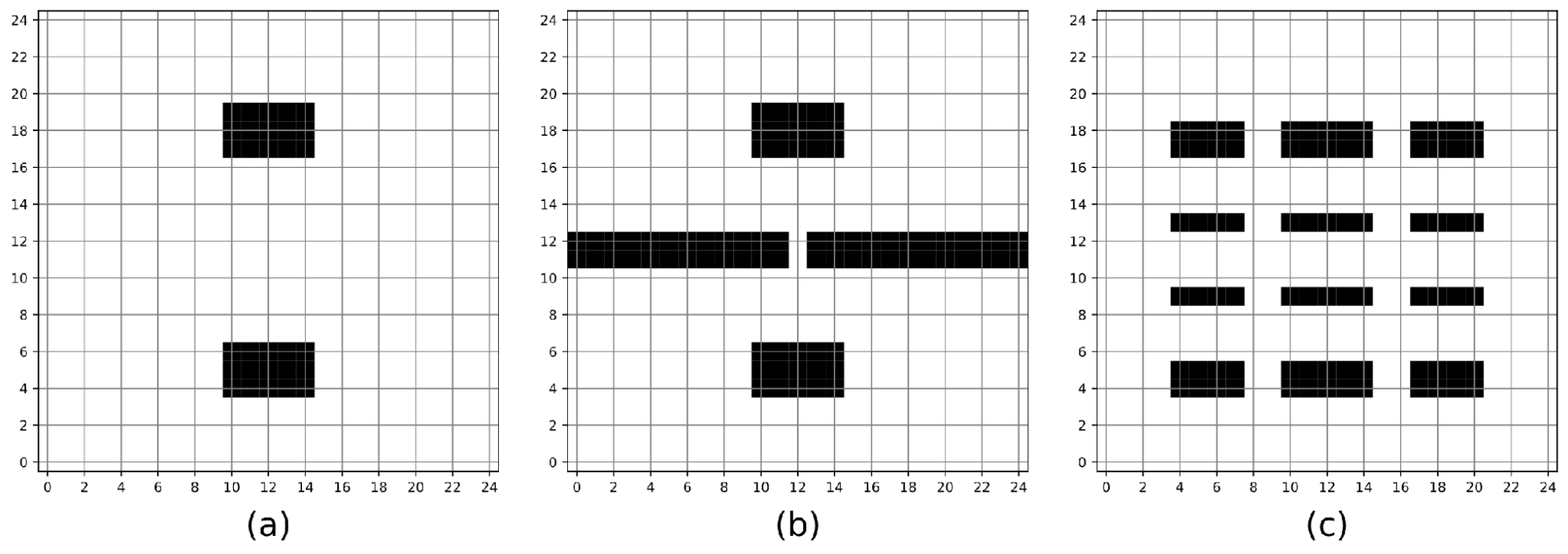
Figure 1. Experimental maps used in this study: (a) Map 1, clustered obstacle layout with open navigation space; (b) Map 2, bottleneck corridor layout with constrained passages; and (c) Map 3, warehouse rack layout with structured aisles
In each experiment, each robot was assigned its own start cell and goal cell randomly selected from the free cells of the respective map; the start-goal set for each experiment was the same for A* and the three NSGA-II formulations to conduct a fair comparison. Since each number of robots constitutes a different scenario, the start-goal set was generated anew whenever the number of robots changed; therefore, robots participating in two scenarios in one and the same map need not have the same start and goal cells. All start-goal sets and seeds used for generating populations are specified.
Each scenario was implemented ten times using fixed random seeds 1 to 10. If no other specification is made, each value used in comparison tables (Table 2 to Table 17) refers to the average over these ten runs; the standard deviations represent the inter-run variability. Both the ten-run statistical campaign and the one-run demonstration campaign were run on the identical Linux workstation as discussed in section 3.7 and used Python 3.12.3, NumPy 2.3.5, SciPy 1.16.3, and pymoo 0.6.1.6. These versions are stated because the seeded evolutionary process, while fully deterministic, is sensitive to the major version of numerical libraries.
Illustrations of representative path comparison, convergence between objective values, and Pareto fronts are shown in Sections 3.2–3.4 using the same visual language that keeps the original A* paths, the three NSGA-II formulations, and the objective space evidence provided in the main text.
Finally, the solution-distribution illustration might have panels based on different visualization techniques, such as 2D or 3D objective space graphs and parallel coordinates graphs. All panels are created using all solutions in the final generation, with non-dominated and dominated solutions being visually separated where possible given the specific graphing technique. The name solution-distribution graph is thus still applicable since the panels will not only help in determining which Pareto front approximation is the preferred one, but also to determine if the last population has become concentrated on the front, become dispersed, or been dominated by infeasible compromises.
Results and Discussion
Experimental results are presented below in this section for all twelve scenarios (two, three, four, and five robots on each of the three maps). Four methods for each scenario are compared: (1) A* (independent decoupled planning), (2) NSGA-II Formulation 1 (aggregated objectives, no constraint), (3) NSGA-II Formulation 2 (per-agent objectives, hard constraint), and (4) NSGA-II Formulation 3 (per-agent objectives, no constraint). All tables provide information about the number of runs with feasible solutions (Feas., n/10), number of collisions (NC), travel time for each robot and total travel time ( ). The termination criteria are summarized in Table 18 (Section 3.6); whether an approach converged early once the hypervolume improvement fell below the preset tolerance or terminated after exhausting maximum generation limit (MaxGen) directly indicates search difficulty of the approach. In order to establish the statistical significance of differences between three formulations, the ten independent runs for each scenario have been tested with non-parametric statistics: Kruskal-Wallis H-test with post-hoc Mann-Whitney U comparisons (Holm-Bonferroni corrected) for TTT and Pareto-front size, and Friedman test with post-hoc Wilcoxon signed-rank comparisons (Holm-Bonferroni corrected) for computation time, as is typical of benchmarking experiments [51].
The Figure 2 to Figure 7 show some of the paths, convergence properties, and Pareto fronts, with each figure showing an example of a different impact. The path and Pareto front graphs in Figure 2 to Figure 4 and Figure 6 to Figure 7 have been derived from the previously designed single-run experiment (seed 1), with a convergence-based budget of up to 250 generations. This set of figures provides an insight into the solution properties, and these figures might include values from the said run, but they are not used for making any statistical comparison or estimating the average performance at 250 generations. Figure 5, on the other hand, represents the same set of ten runs of fixed budget (100 generations) that has been presented in the tables above.
Scenario Performance Summary
Table 2 to Table 4 summarize the two-robot scenarios. The decoupled A* baseline remains collision-free on all three maps, and all three NSGA-II formulations are fully feasible in every run while reducing the TTT relative to A* on the clustered, bottleneck, and warehouse layouts alike. The three formulations reach statistically equivalent travel times at this scale (Section 3.5), so formulation design has little influence when coordination pressure is low. Table 5 to Table 7 report the three-robot scenarios, where the A* baseline starts to accumulate collisions on Maps 1 and 2. Formulations 1 and 2 remain fully feasible in all runs and continue to improve the TTT. Formulation 3 begins to weaken: its feasibility rate declines and its feasible runs carry higher travel times on Maps 1 and 2 (Section 3.5), while on Map 3 all three formulations remain close.
Table 2. Comparison of path planning performance on Map 1 with two robots
Algorithm/Formulation | Feas. (n/10) | NC | T1 | T2 | TTT |
A* (independent, reference) | — | 0 | 44 | 44 | 88 |
NSGA-II (Form. 1 – AGG) | 10/10 | 0.0 ± 0.0 | 36.5 ± 0.5 | 36.5 ± 0.5 | 73.0 ± 0.0 |
NSGA-II (Form. 2 – AWC) | 10/10 | 0.0 ± 0.0 | 36.4 ± 0.5 | 36.6 ± 0.5 | 73.0 ± 0.0 |
NSGA-II (Form. 3 – AWOC) | 10/10 | 0.0 ± 0.0 | 36.6 ± 0.5 | 36.4 ± 0.5 | 73.0 ± 0.0 |
Values are mean ± SD over 10 independent runs (seeds 1–10), taken from the preferred feasible solution of each run. Feas. (n/10): number of feasible runs out of 10 (NC = 0, residual distance = 0). NC: number of collisions, mean ± SD over all 10 runs.  .. .. : per-robot travel time in discrete time units under the unit-duration setting of Equation (6). TTT: total travel time = ΣTr; Ti and TTT are mean ± SD over feasible runs only (± 0.0 when all feasible runs yield the same value). A* is a single deterministic reference run with independently planned per-robot paths (no collision resolution). —: Ti and TTT are omitted for Form. 3 (AWOC) when fewer than 5 runs are feasible; Feas. and NC remain reported. These conventions apply to Table 2 to Table 13 : per-robot travel time in discrete time units under the unit-duration setting of Equation (6). TTT: total travel time = ΣTr; Ti and TTT are mean ± SD over feasible runs only (± 0.0 when all feasible runs yield the same value). A* is a single deterministic reference run with independently planned per-robot paths (no collision resolution). —: Ti and TTT are omitted for Form. 3 (AWOC) when fewer than 5 runs are feasible; Feas. and NC remain reported. These conventions apply to Table 2 to Table 13 |
.
Table 3. Comparison of path planning performance on Map 2 with two robots
Algorithm/Formulation | Feas. (n/10) | NC | T1 | T2 | TTT |
A* (independent, reference) | — | 0 | 54 | 44 | 98 |
NSGA-II (Form. 1 – AGG) | 10/10 | 0.0 ± 0.0 | 40.3 ± 0.7 | 39.5 ± 0.8 | 79.8 ± 0.6 |
NSGA-II (Form. 2 – AWC) | 10/10 | 0.0 ± 0.0 | 39.7 ± 0.9 | 40.0 ± 0.9 | 79.7 ± 0.5 |
NSGA-II (Form. 3 – AWOC) | 10/10 | 0.0 ± 0.0 | 39.8 ± 0.9 | 40.1 ± 1.1 | 79.9 ± 0.6 |
Table 4. Comparison of path planning performance on Map 3 with two robots
Algorithm/Formulation | Feas. (n/10) | NC | T1 | T2 | TTT |
A* (independent, reference) | — | 0 | 61 | 50 | 111 |
NSGA-II (Form. 1 – AGG) | 10/10 | 0.0 ± 0.0 | 41.5 ± 0.5 | 41.5 ± 0.5 | 83.0 ± 0.0 |
NSGA-II (Form. 2 – AWC) | 10/10 | 0.0 ± 0.0 | 41.5 ± 0.5 | 41.5 ± 0.5 | 83.0 ± 0.0 |
NSGA-II (Form. 3 – AWOC) | 10/10 | 0.0 ± 0.0 | 41.3 ± 0.5 | 41.7 ± 0.5 | 83.0 ± 0.0 |
Table 5. Comparison of path planning performance on Map 1 with three robots
Algorithm/Formulation | Feas. (n/10) | NC | T1 | T2 | T3 | TTT |
A* (independent, reference) | — | 1 | 44 | 44 | 34 | 122 |
NSGA-II (Form. 1 – AGG) | 10/10 | 0.0 ± 0.0 | 37.1 ± 1.0 | 36.3 ± 0.5 | 29.2 ± 0.6 | 102.6 ± 0.8 |
NSGA-II (Form. 2 – AWC) | 10/10 | 0.0 ± 0.0 | 36.4 ± 0.5 | 36.6 ± 0.5 | 29.0 ± 0.0 | 102.0 ± 0.0 |
NSGA-II (Form. 3 – AWOC) | 10/10 | 0.0 ± 0.0 | 37.7 ± 1.9 | 37.5 ± 2.4 | 30.3 ± 2.8 | 105.5 ± 5.3 |
Table 6. Comparison of path planning performance on Map 2 with three robots
Algorithm/Formulation | Feas. (n/10) | NC | T1 | T2 | T3 | TTT |
A* (independent, reference) | — | 1 | 54 | 44 | 45 | 143 |
NSGA-II (Form. 1 – AGG) | 10/10 | 0.0 ± 0.0 | 41.4 ± 1.4 | 41.2 ± 1.3 | 39.5 ± 1.3 | 122.1 ± 1.0 |
NSGA-II (Form. 2 – AWC) | 10/10 | 0.0 ± 0.0 | 41.4 ± 1.6 | 41.2 ± 1.2 | 40.1 ± 1.4 | 122.7 ± 0.9 |
NSGA-II (Form. 3 – AWOC) | 8/10 | 0.4 ± 1.0 | 56.4 ± 14.1 | 63.0 ± 12.6 | 56.6 ± 7.6 | 176.0 ± 10.4 |
Table 7. Comparison of path planning performance on Map 3 with three robots
Algorithm/Formulation | Feas. (n/10) | NC | T1 | T2 | T3 | TTT |
A* (independent, reference) | — | 0 | 61 | 50 | 22 | 133 |
NSGA-II (Form. 1 – AGG) | 10/10 | 0.0 ± 0.0 | 41.4 ± 0.5 | 41.6 ± 0.5 | 22.0 ± 0.0 | 105.0 ± 0.0 |
NSGA-II (Form. 2 – AWC) | 10/10 | 0.0 ± 0.0 | 41.8 ± 0.4 | 41.2 ± 0.4 | 22.0 ± 0.0 | 105.0 ± 0.0 |
NSGA-II (Form. 3 – AWOC) | 10/10 | 0.0 ± 0.0 | 41.6 ± 0.7 | 41.8 ± 1.0 | 23.2 ± 2.5 | 106.6 ± 2.9 |
Table 8 to Table 10 deals with the four-robot cases. The feasibility and statistical equivalence of Formulations 1 and 2 remain the same in the TTT (Section 3.5). Among all the three formulations, Formulation 2 generates the most compact Pareto fronts (see Table 16). Formulation 3 has become the worst choice because of its low feasibility ratio and high feasible numbers. Five robots formulations (Table 11 to Table 13) form the most difficult cases. Formulations 1 and 2 still retain their full feasibility, while Formulation 3 loses its feasibility since only one or two iterations are feasible.
Table 8. Comparison of path planning performance on Map 1 with four robots
Algorithm/Formulation | Feas. (n/10) | NC | T1 | T2 | T3 | T4 | TTT |
A* (independent, reference) | — | 0 | 44 | 44 | 34 | 33 | 155 |
NSGA-II (Form. 1 – AGG) | 10/10 | 0.0 ± 0.0 | 36.9 ± 1.2 | 36.6 ± 1.0 | 29.8 ± 0.6 | 29.4 ± 0.5 | 132.7 ± 1.3 |
NSGA-II (Form. 2 – AWC) | 10/10 | 0.0 ± 0.0 | 36.6 ± 0.7 | 37.0 ± 1.2 | 29.9 ± 0.7 | 29.5 ± 0.5 | 133.0 ± 1.2 |
NSGA-II (Form. 3 – AWOC) | 8/10 | 0.7 ± 1.6 | 45.8 ± 10.9 | 49.2 ± 7.9 | 44.2 ± 13.0 | 39.6 ± 10.0 | 178.9 ± 29.8 |
Table 9. Comparison of path planning performance on Map 2 with four robots
Algorithm/Formulation | Feas. (n/10) | NC | T1 | T2 | T3 | T4 | TTT |
A* (independent, reference) | — | 4 | 54 | 44 | 41 | 37 | 176 |
NSGA-II (Form. 1 – AGG) | 10/10 | 0.0 ± 0.0 | 42.4 ± 1.0 | 41.7 ± 0.7 | 35.8 ± 1.0 | 36.1 ± 1.0 | 156.0 ± 1.2 |
NSGA-II (Form. 2 – AWC) | 10/10 | 0.0 ± 0.0 | 42.0 ± 1.3 | 41.8 ± 1.3 | 36.3 ± 0.9 | 36.0 ± 1.9 | 156.1 ± 1.0 |
NSGA-II (Form. 3 – AWOC) | 3/10 | 3.8 ± 4.4 | — | — | — | — | — |
Table 10. Comparison of path planning performance on Map 3 with four robots
Algorithm/Formulation | Feas. (n/10) | NC | T1 | T2 | T3 | T4 | TTT |
A* (independent, reference) | — | 0 | 61 | 50 | 22 | 22 | 155 |
NSGA-II (Form. 1 – AGG) | 10/10 | 0.0 ± 0.0 | 41.5 ± 0.5 | 41.6 ± 0.7 | 22.0 ± 0.0 | 22.0 ± 0.0 | 127.1 ± 0.3 |
NSGA-II (Form. 2 – AWC) | 10/10 | 0.0 ± 0.0 | 41.5 ± 0.5 | 41.5 ± 0.5 | 22.0 ± 0.0 | 22.0 ± 0.0 | 127.0 ± 0.0 |
NSGA-II (Form. 3 – AWOC) | 10/10 | 0.0 ± 0.0 | 45.0 ± 4.6 | 44.2 ± 5.0 | 23.0 ± 3.2 | 22.0 ± 0.0 | 134.2 ± 11.6 |
Table 11. Comparison of path planning performance on Map 1 with five robots
Algorithm/Formulation | Feas. (n/10) | NC | T1 | T2 | T3 | T4 | T5 | TTT |
A* (independent, reference) | — | 3 | 44 | 44 | 34 | 33 | 34 | 189 |
NSGA-II (Form. 1 – AGG) | 10/10 | 0.0 ± 0.0 | 37.0 ± 1.3 | 37.2 ± 1.4 | 30.4 ± 1.0 | 29.5 ± 1.0 | 29.8 ± 1.0 | 163.9 ± 2.1 |
NSGA-II (Form. 2 – AWC) | 10/10 | 0.0 ± 0.0 | 38.2 ± 3.2 | 40.0 ± 2.8 | 30.0 ± 0.9 | 31.8 ± 2.2 | 31.0 ± 2.3 | 171.0 ± 3.5 |
NSGA-II (Form. 3 – AWOC) | 2/10 | 8.1 ± 9.7 | — | — | — | — | — | — |
Table 12. Comparison of path planning performance on Map 2 with five robots
Algorithm/Formulation | Feas. (n/10) | NC | T1 | T2 | T3 | T4 | T5 | TTT |
A* (independent, reference) | — | 6 | 54 | 44 | 41 | 37 | 45 | 221 |
NSGA-II (Form. 1 – AGG) | 10/10 | 0.0 ± 0.0 | 44.1 ± 3.0 | 44.1 ± 1.7 | 35.8 ± 1.1 | 36.5 ± 1.4 | 43.8 ± 1.9 | 204.3 ± 4.2 |
NSGA-II (Form. 2 – AWC) | 10/10 | 0.0 ± 0.0 | 47.1 ± 3.9 | 45.1 ± 3.7 | 36.6 ± 1.3 | 37.5 ± 3.5 | 44.5 ± 2.9 | 210.8 ± 3.3 |
NSGA-II (Form. 3 – AWOC) | 1/10 | 6.5 ± 4.7 | — | — | — | — | — | — |
Table 13. Comparison of path planning performance on Map 3 with five robots
Algorithm/Formulation | Feas. (n/10) | NC | T1 | T2 | T3 | T4 | T5 | TTT |
A* (independent, reference) | — | 7 | 36 | 36 | 35 | 37 | 30 | 174 |
NSGA-II (Form. 1 – AGG) | 10/10 | 0.0 ± 0.0 | 36.4 ± 0.7 | 36.9 ± 0.7 | 30.4 ± 0.5 | 31.0 ± 0.9 | 30.9 ± 1.1 | 165.6 ± 1.3 |
NSGA-II (Form. 2 – AWC) | 10/10 | 0.0 ± 0.0 | 39.0 ± 4.1 | 39.2 ± 2.3 | 31.1 ± 1.2 | 32.1 ± 2.8 | 31.2 ± 1.6 | 172.6 ± 3.8 |
NSGA-II (Form. 3 – AWOC) | 2/10 | 1.2 ± 0.8 | — | — | — | — | — | — |
Representative Path Behavior
Path behavior is illustrated with three representative scenarios spanning the difficulty range; the remaining scenarios exhibit similar qualitative patterns, and their complete quantitative results are given in Table 2 to Table 13. Figure 2 shows the easiest instance, two robots on Map 1. The initial A* paths are already collision-free but suboptimal in TTT: Formulation 1 reduces the total from 88 to 75, and Formulations 2 and 3 both improve further to 73, so the per-agent formulations produce the best feasible timing allocation in this low-interaction setting.
Figure 3 shows the three-robot bottleneck case on Map 2, where the initial A* paths already contain collisions. Formulation 1 resolves them and reduces the TTT from 143 to 121, and Formulation 2 reaches a nearby collision-free result at 122, whereas Formulation 3 ends at 154, worse than the total produced by the initial A* paths. This illustrates how the unconstrained per-agent design begins to lose practical reliability once coordination pressure rises.
Figure 4 shows the five-robot warehouse case on Map 3, the most contested instance in the study. The initial A* paths accumulate 14 collisions with a TTT of 174, while Formulation 1 removes all collisions and lowers the total to 165. Formulation 2 performs slightly better at 164, whereas Formulation 3 remains worse than the initial A* total at 191 and still retains two collisions.
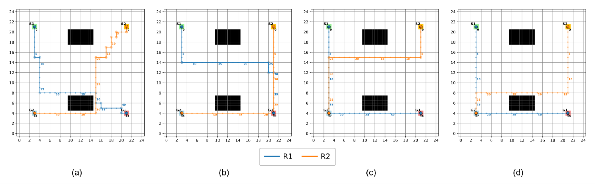
Figure 2. Path comparison on Map 1 with two robots: (a) A*; (b) NSGA-II Formulation 1; (c) NSGA-II Formulation 2; and (d) NSGA-II Formulation 3
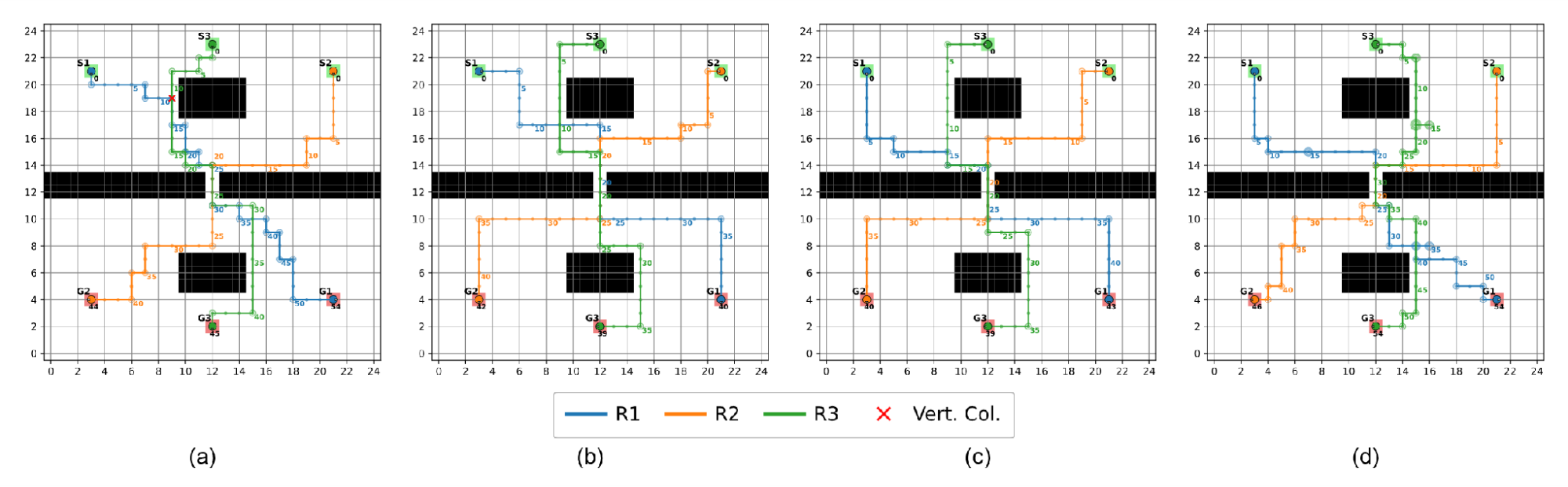
Figure 3. Path comparison on Map 2 with three robots: (a) A*; (b) NSGA-II Formulation 1.; (c) NSGA-II Formulation 2; and (d) NSGA-II Formulation 3
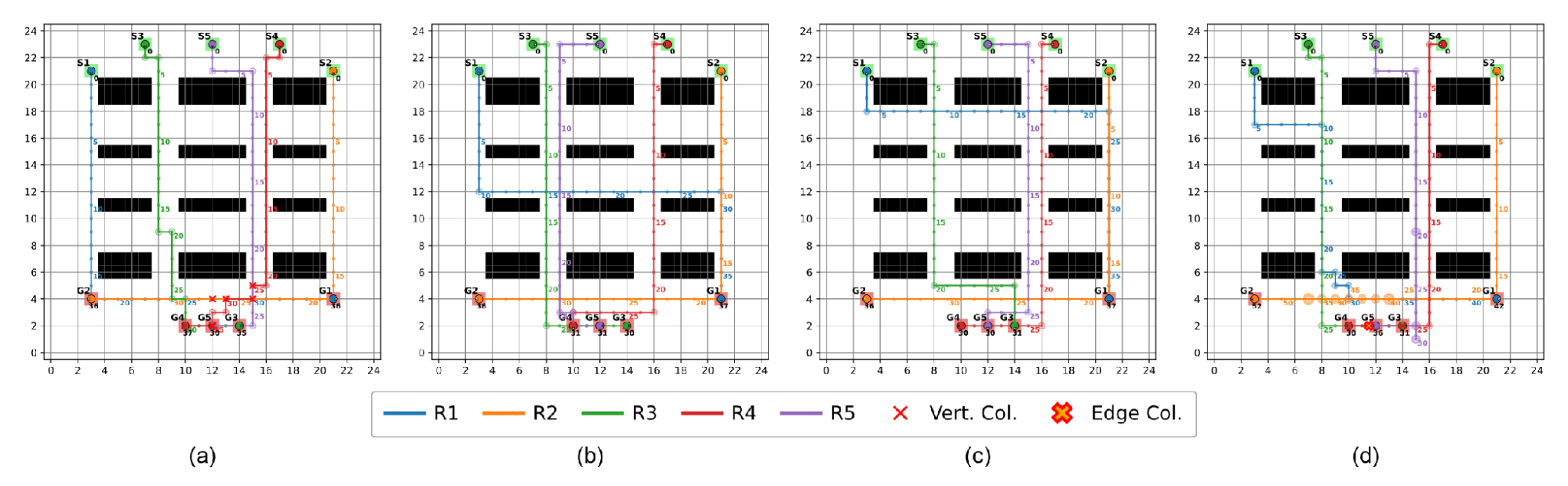
Figure 4. Path comparison on Map 3 with five robots: (a) A*; (b) NSGA-II Formulation 1.; (c) NSGA-II Formulation 2; and (d) NSGA-II Formulation 3
Convergence Behavior
The convergence trend is indicated by plotting the normalized hypervolume (HV) through generations, which shows the evolution of the front in an ongoing manner [52], within the shared objective space described in Section 3.5, for a small and a large instance (Figure 5; average from ten seeds, min-max shaded range, constant budget of 100 generations). For the two robots on Map 1, the three formulations quickly increase to 30 generations; after that, Formulation 2 stagnates at its feasible optimal point, while Formulations 1 and 3 continue to expand their trade-off fronts.
In case of five robots in a warehouse environment, formulation one increases in monotonic fashion until it achieves the maximum plateau. On the other hand, Formulation 2 gradually moves towards a viable optimum solution. However, Formulation 3 achieves its maximum at generation 30 and then starts decreasing, which shows the lack of diversity because of the crowding distance selection technique. Under the separate convergence-based budget of up to 250 generations, this scenario is also the most termination-resistant instance in the study: none of the three formulations converge. The termination condition for every scenario and formulation is summarized in Table 18 (Section 3.6), and runtime is analyzed in Section 3.7.
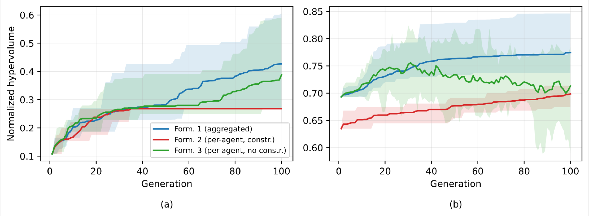
Figure 5. Normalized hypervolume versus generation in the common objective space: (a) Map 1, two robots; (b) Map 3, five robots. Lines show the mean of ten seeds; shaded bands the min-max range (10 runs, fixed budget of 100 generations)
Pareto-Front Structure and Interpretability
Figure 6 shows the final solution distributions for the two-robot case on Map 1. Formulation 1 stabilizes around a very small aggregated front with a narrow objective span from  = 72 to 75, whose lowest-travel-time member is still collision-prone. Formulation 2 collapses to two symmetric feasible compromises, (36, 37) and (37, 36), while Formulation 3 remains similarly compact with five Pareto members, four of which are soft-feasible. The per-agent formulations therefore expose the same narrow feasible trade-off structure more cleanly than the aggregated view.
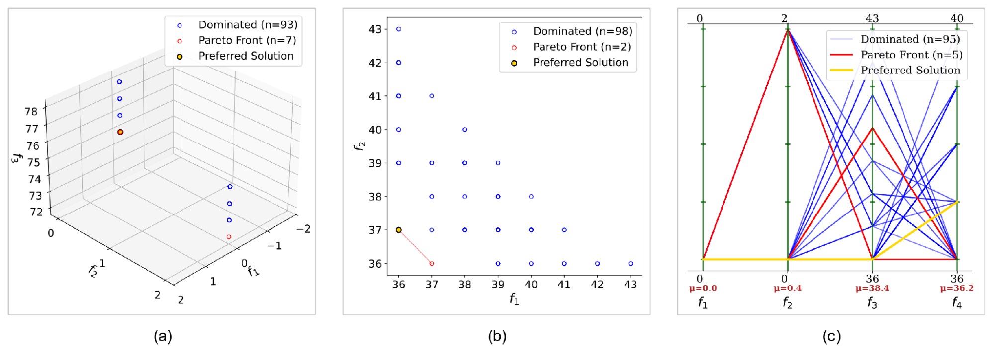
Figure 6. Pareto-front approximation on Map 1 with two robots: (a) Form. 1, (b) Form. 2, and (c) Form. 3
Figure 7 shows the five-robot warehouse case. Formulation 1 leaves all 100 final-generation points non-dominated with only two soft-feasible members and a very wide aggregate range from = 120 to 165. Formulation 2 reduces this to a much tighter feasible frontier of 22 Pareto members with moderate spreads across all five travel-time axes, whereas Formulation 3 leaves all 100 points non-dominated with none soft-feasible. Only the constrained per-agent formulation turns the final population into a directly usable set of deployment alternatives.
This is due to the common problem encountered in Pareto-dominance based algorithms like NSGA-II when the number of objectives becomes more than three; the dominance pressure decreases very quickly [53] [54] thereby limiting the efficiency of the algorithm in guiding the population towards the genuine Pareto-optimal frontier. Several many-objective evolutionary algorithms have been proposed to address this limitation, including reference-point-based methods such as NSGA-III [55], decomposition-based approaches such as MOEA/D [56], indicator-based algorithms [57], adaptive reference-vector methods [58], and angle- or geometry-based selection strategies [59].
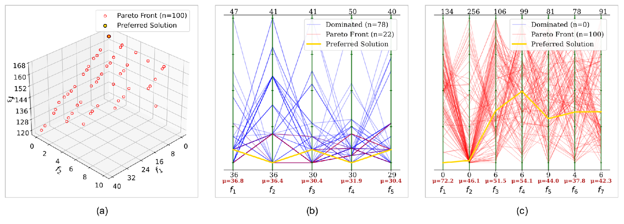
Figure 7. Pareto-front approximation on Map 3 with five robots: (a) Form. 1, (b) Form. 2, and (c) Form. 3
Statistical Comparison of Formulations
To substantiate the per-scenario observations in Section 3.1, the three formulations were compared statistically using 10 independent runs (seeds 1-10) per scenario, each with a fixed budget of 100 generations. A Kruskal-Wallis H-test was applied per scenario block to test for differences in TTT; where it was significant (alpha = 0.05), pairwise Mann-Whitney U tests were run for the three pairs (AGG-AWC, AGG-AWOC, AWC-AWOC) with Holm-Bonferroni correction. Only feasible runs (NC = 0, zero residual distance) entered the TTT analysis.
For two-robot scenarios (R = 2), no significant differences were found on any map, so all formulations reach equivalent solutions under low-complexity conditions. For three- and four-robot scenarios, the Kruskal-Wallis test was significant in all six blocks; the post-hoc tests identify AWOC as the weaker formulation (the post-hoc tests identify AWOC as the weaker formulation (AWC-AWOC significant after Holm in all five remaining blocks and AGG-AWOC in four of the five, with AWOC median TTT higher by 3 to 55 steps), while AGG and AWC never differ significantly. The sole exception here is R = 3, Map 3, where the Kruskal-Wallis test yields significance but none of pairs withstands Holm correction; in that case AWOC is still completely feasible and median TTT of AWOC is slightly higher. In case of five-robots scenario AGG demonstrates significantly lower median TTT than AWC on all three maps (p = 0.0007-0.0062 after Holm), which equals 5 to 7 steps; AWOC was impossible to assess reliably in R = 5 due to lack of feasibility of 1 to 2 out of 10 runs.
Kruskal-Wallis test on Pareto-front size proves to be significant in 10 of 12 blocks. AWOC achieves population limit of 100 non-dominated solutions in all scenarios involving three or more robots; it means that this Pareto front includes infeasible solutions only, whereas the rest are dominated ones; AWC generates the least distributed front in three and four robots' cases. In light of this information, the following can be stated: all formulations are equally effective in R = 2; AWOC is less efficient in terms of feasibility and TTT than other formulations for three or more robots; and finally, AGG and AWC demonstrate statistical equivalence in terms of TTT up to four robots inclusively, and slight advantage of AGG in R = 5. Therefore, AWC is the preferable formulation among others considered in this study because of full feasibility in all scenarios and understandable trade-offs per agent.
Table 15 provides the feasibility percentage. Formulations 1 and 2 still maintain their 100% feasibility in all cases, but Formulation 3 achieves only 1 out of 10 feasible runs at five robots. Table 16 gives the median number of points on the Pareto front. Formulation 3 reaches the population cap of 100 points in every four- and five-robot scenario (and at R = 3 on Map 2), approaching it at R = 3 on the other two maps, but Formulation 2 maintains the tightest front; the Kruskal-Wallis p-value compares the three formulations across scenarios.
The comparisons above concern deployment-oriented quantities (feasibility, TTT, and Pareto-front size). To assess the quality of the approximation fronts themselves, two standard indicators are additionally reported: hypervolume (HV), the only unary indicator fully compliant with Pareto dominance [60], and the inverted generational distance (IGD) [57]. Because the three formulations optimize objective vectors of different dimensionality (M = 3, R, and R + 2), indicator values computed in each formulation's own objective space are not mutually comparable. All final populations are therefore projected into a common three-dimensional space, the sum of residual distances (), the number of inter-agent collisions (), and the TTT (), in which every solution of every formulation is well defined; the projection is exact and requires no re-evaluation. For each scenario, the HV reference point is set to 1.10 times the per-objective maximum over the union of all 30 runs (3 formulations × 10 seeds), HV values are normalized by the volume between this reference point and the union ideal point, and the IGD reference front is the non-dominated subset of the union of all 30 run fronts, computed on objectives normalized to the same range. Differences across formulations are tested per scenario with the Kruskal-Wallis test (α = 0.05).
Table 14. Kruskal-Wallis p-values and Holm-adjusted pairwise p-values for feasible-run total travel time (TTT)
NR | Map | 
| AGG-AWC ( ) ) | AGG-AWOC () | AWC-AWOC () |
2 | 1 | n/a | — | — | — |
2 | 0.74405 | — | — | — |
3 | n/a | — | — | — |
3 | 1 | 0.01006 | 0.06941 | 0.11338 | 0.01775 |
2 | 0.00012 | 0.22847 | 0.00108 | 0.00080 |
3 | 0.01184 | 1.00000 | 0.10453 | 0.06969 |
4 | 1 | 0.00011 | 0.33470 | 0.00089 | 0.00077 |
2 | 0.01767 | 0.81138 | 0.03472 | 0.02438 |
3 | <0.001 | 0.36812 | 0.00012 | 0.00012 |
5 | 1 | 0.00024 | 0.00071 | † | † |
2 | 0.00181 | 0.00618 | † (1/10) | † |
3 | 0.00028 | 0.00086 | † | † |
NR: Number of Robots; is the omnibus Kruskal-Wallis p-value. Pairwise values are Holm-Bonferroni-adjusted p-values. Values significant at ( ) are shown in bold. — = post-hoc comparison not performed after a non-significant omnibus test; n/a = all values identical (no variance to test); † = (n_ ) are shown in bold. — = post-hoc comparison not performed after a non-significant omnibus test; n/a = all values identical (no variance to test); † = (n_ ), so pairwise inference is unreliable and excluded from claims. ), so pairwise inference is unreliable and excluded from claims. |
Table 15. Feasibility rate (feasible runs out of 10) for the three formulations across all scenarios
Map | NR | Form. 1 (AGG) | Form. 2 (AWC) | Form. 3 (AWOC) |
1 | 2 | 10/10 | 10/10 | 10/10 |
3 | 10/10 | 10/10 | 10/10 |
4 | 10/10 | 10/10 | 8/10 |
5 | 10/10 | 10/10 | 2/10 |
2 | 2 | 10/10 | 10/10 | 10/10 |
3 | 10/10 | 10/10 | 8/10 |
4 | 10/10 | 10/10 | 3/10 |
5 | 10/10 | 10/10 | 1/10 |
3 | 2 | 10/10 | 10/10 | 10/10 |
3 | 10/10 | 10/10 | 10/10 |
4 | 10/10 | 10/10 | 10/10 |
5 | 10/10 | 10/10 | 2/10 |
Table 16. Median Pareto-front size per run, with the Kruskal-Wallis p-value per scenario
Map | NR | Form. 1 (AGG) | Form. 2 (AWC) | Form. 3 (AWOC) | KW p |
1 | 2 | 38.0 | 9.0 | 5.5 | n.s. |
3 | 91.5 | 23.0 | 89.5 | <0.001 |
4 | 4.0 | 3.5 | 100.0 | <0.001 |
5 | 7.0 | 42.0 | 100.0 | <0.001 |
2 | 2 | 21.0 | 28.0 | 67.0 | 0.010 |
3 | 65.0 | 16.5 | 100.0 | <0.001 |
4 | 54.0 | 21.5 | 100.0 | <0.001 |
5 | 21.5 | 63.5 | 100.0 | <0.001 |
3 | 2 | 18.0 | 7.0 | 18.0 | n.s. |
3 | 5.0 | 4.5 | 98.5 | <0.001 |
4 | 6.5 | 3.5 | 100.0 | <0.001 |
5 | 22.5 | 43.0 | 100.0 | <0.001 |
Table 17 summarizes the results; the differences are significant in all twelve scenarios for both indicators. Formulation 3 attains the largest HV and the smallest IGD in most scenarios with two to four robots, whereas Formulation 1 leads in all five-robot scenarios; Formulation 2 yields the lowest HV throughout. These indicators must, however, be read together with the deployment metrics: HV and IGD reward broad coverage of the projected objective space, including trade-off solutions that still contain collisions ( > 0), which Formulations 1 and 3 retain in their populations by design. Formulation 2 instead concentrates its search on the feasible region ( = = 0), so its projected front collapses toward the single best feasible travel time, a small hypervolume, but the highest feasibility rates in Table 15. Indeed, in several small scenarios Formulation 2 reaches an identical feasible optimum in all ten seeds (zero variance), indicating deterministic reliability rather than poor search. The five-robot pattern is consistent with the termination analysis in Table 18: under a fixed generation budget, the fixed three-dimensional space of Formulation 1 is easier to cover than the seven-dimensional per-agent spaces. The generation-wise behavior of HV underlying these end-of-run values is shown in Figure 5 (Section 3.3).
Table 17. Normalized hypervolume (HV, higher is better) and inverted generational distance (IGD, lower is better) in the common objective space (mean ± SD over 10 runs), with Kruskal-Wallis p-values per scenario
NR | Map | HV Form. 1 | HV Form. 2 | HV Form. 3 | KW p (HV) | IGD Form. 1 | IGD Form. 2 | IGD Form. 3 | KW p (IGD) |
2 | 1 | 0.43±0.12 | 0.27±0.00 | 0.39±0.11 | <0.001 | 0.018±0.011 | 0.315±0.000 | 0.022±0.010 | <0.001 |
2 | 0.26±0.03 | 0.24±0.01 | 0.49±0.09 | <0.001 | 0.301±0.055 | 0.353±0.004 | 0.088±0.047 | <0.001 |
3 | 0.52±0.09 | 0.42±0.00 | 0.56±0.08 | <0.001 | 0.013±0.008 | 0.042±0.000 | 0.010±0.007 | <0.001 |
3 | 1 | 0.57±0.02 | 0.49±0.00 | 0.73±0.03 | <0.001 | 0.034±0.007 | 0.093±0.000 | 0.031±0.033 | <0.001 |
2 | 0.60±0.00 | 0.57±0.00 | 0.74±0.01 | <0.001 | 0.157±0.005 | 0.181±0.003 | 0.121±0.015 | <0.001 |
3 | 0.46±0.07 | 0.41±0.00 | 0.68±0.03 | <0.001 | 0.086±0.033 | 0.116±0.000 | 0.016±0.009 | <0.001 |
4 | 1 | 0.70±0.03 | 0.67±0.00 | 0.74±0.02 | <0.001 | 0.049±0.011 | 0.059±0.004 | 0.131±0.058 | <0.001 |
2 | 0.62±0.01 | 0.60±0.00 | 0.68±0.04 | <0.001 | 0.363±0.007 | 0.389±0.001 | 0.117±0.027 | <0.001 |
3 | 0.64±0.01 | 0.62±0.00 | 0.73±0.03 | <0.001 | 0.052±0.008 | 0.060±0.000 | 0.037±0.026 | <0.001 |
5 | 1 | 0.78±0.03 | 0.73±0.01 | 0.74±0.04 | 0.002 | 0.106±0.036 | 0.151±0.007 | 0.214±0.050 | <0.001 |
2 | 0.79±0.05 | 0.68±0.01 | 0.76±0.03 | <0.001 | 0.111±0.065 | 0.213±0.007 | 0.212±0.040 | <0.001 |
3 | 0.77±0.03 | 0.70±0.01 | 0.71±0.06 | <0.001 | 0.044±0.014 | 0.097±0.010 | 0.190±0.079 | <0.001 |
HV and IGD are computed in the common objective space (, , ); shared reference point per scenario = 1.10 × per-objective maximum over all 30 runs; KW p = Kruskal-Wallis p-value across the three formulations (α = 0.05). |
Summary of Termination Behavior
The termination summary across the twelve planning scenarios shows a clear scaling effect with respect to both robot count and map structure. All three formulations converge in the two-robot cases, and Formulations 1 and 2 remain convergent across all three-robot cases. Beyond that point, convergence becomes increasingly difficult: only some four-robot cases still satisfy the hypervolume criterion within the 250-generation budget, and the five-robot Map 3 scenario does not converge for any formulation. These results indicate that the current budget is generally sufficient at low-to-moderate scale but becomes restrictive as coordination density increases.
When comparing termination across formulations, it should be noted that the hypervolume-based stopping rule is applied in objective spaces of different dimensionality (three for Formulation 1, R for Formulation 2, and R+2 for Formulation 3). Moreover, dominance-based selection in NSGA-II is known to weaken once the number of objectives exceeds three to four, which slows the stabilization of the hypervolume indicator independently of the underlying search progress. Therefore, the reported termination results reflect the convergence behavior of each formulation under its own stopping criterion rather than a direct comparison across formulations. Some of Formulation 3's non-convergent (MaxGen) runs may therefore reflect the higher-dimensional objective space rather than search failure alone.
The sharp degradation of Formulation 3 at four and five robots should be interpreted with care, because two effects are confounded by design. Formulation 3 removes the hard constraints, but it also has the highest objective dimensionality (R+2, i.e., up to seven objectives at five robots), whereas Formulation 2 shares the per-agent structure yet keeps only R objectives and remains fully feasible. The primary driver of Formulation 3's collapse is the loss of feasibility that follows from removing the constraints; in addition, because NSGA-II relies on Pareto dominance, whose selection pressure is known to weaken beyond three or four objectives [53][54], the many-objective setting compounds the degradation. Isolating these two causes would require running the per-agent formulations under a many-objective engine designed for high-dimensional objective spaces, such as a reference-point method (NSGA-III [54][55]) or a decomposition-based method (MOEA/D [56]); if Formulation 3 recovered under such an engine while Formulation 2 remained stable, dimensionality would be implicated, whereas persistent failure would strengthen the constraint-absence explanation. The comparative analysis described above is left for future work, and the current observations on Formulation 3 are presented here as results based on NSGA-II rather than as general claims regarding the formulation.
These findings are in agreement with earlier research on NSGA-II-based path-planning algorithms, wherein A* seeding speeds up the algorithm's convergence rate [27], and multi-objective problem formulations offer more tradeoffs than aggregations of single objectives [28][29]. As the former studies have used distinct maps, numbers of robots, and objective functions, a numerical comparison does not make sense; however, the latter constitutes the contribution of this work.
The termination condition is reported from a single illustrative run per scenario with a convergence-based budget of up to 250 generations and therefore complements Table 2 to Table 13, which aggregate ten independent runs with a fixed budget of 100 generations. Each cell in Table 18 reports the generation at which the hypervolume criterion was met; shaded cells marked with an asterisk reached the maximum generation limit (250) without converging (MaxGen).
Table 18. Termination condition (generation at convergence or MaxGen limit) for each map, robot count, and formulation. Shaded cells indicate runs that failed to converge within 250 generations
NR | Map | Form. 1 (AGG) | Form. 2 (AWC) | Form. 3 (AWOC) |
2 | 1 | 37 | 44 | 62 |
2 | 82 | 66 | 124 |
3 | 45 | 49 | 56 |
3 | 1 | 53 | 67 | 250* |
2 | 130 | 181 | 250* |
3 | 32 | 66 | 247 |
4 | 1 | 250* | 104 | 250* |
2 | 90 | 250* | 250* |
3 | 38 | 68 | 250* |
5 | 1 | 101 | 219 | 250* |
2 | 169 | 250* | 250* |
3 | 250* | 250* | 250* |
* Reached the maximum generation limit (250) without converging (MaxGen). |
Formulation 1 exhibits the most stable termination behavior overall. It converges in 10 of 12 scenarios, covering all two-robot and three-robot cases, two four-robot cases (Map 2 at generation 90 and Map 3 at generation 38), and two five-robot cases (Map 1 at generation 101 and Map 2 at generation 169). Its only non-convergent cases are Map 1 with four robots and Map 3 with five robots, indicating that the aggregated-objective formulation remains the most robust as the search space grows.
Formulation 2 converges in 9 of 12 scenarios. Like Formulation 1, it converges in all two-robot and three-robot cases, but it generally stabilizes later, most notably on Map 2 with three robots (generation 181) and Map 1 with five robots (generation 219). At higher robot counts, its convergence becomes less consistent: it converges on Map 1 and Map 3 with four robots and on Map 1 with five robots but reaches MaxGen in the remaining larger cases. From these results, one can say that handling hard constraints maintains feasibility but makes satisfaction of the hypervolume-based termination criterion harder.
Formulation 3 demonstrates the worst termination performance among the three formulations. It stabilizes only in the three cases when there are two robots and in the case of three robots in Map 3. Stabilization in the latter case comes rather late, at generation 247. In other eight scenarios, it reaches MaxGen. Overall, in their individual hypervolume stopping conditions, the stability of termination occurs in the order of Formulation 1, Formulation 2, and Formulation 3. The unconstrained formulation for each agent is more difficult to terminate as the degree of coordination increases.
Computational Time Analysis
The computation time was recorded on ten independent experiments per scenario configuration on an Intel Xeon CPU E5-2697 v4 @ 2.30 GHz, 8 cores, 7.8 GB RAM, Ubuntu 24.04.2 LTS, and Python 3.12.3 with NumPy 2.3.5, SciPy 1.16.3, and pymoo 0.6.1.6. Convergence detection was turned off and the generation budget was set to MaxGen = 100 in all scenarios to guarantee equality of the number of generations for comparison between different maps, robot counts, and formulations.
Table 19 shows computational time statistics for twelve map-robot configuration scenarios for three formulations. The mean execution time varies from 70.96 seconds (Formulation 3, Map 2, 2 robots) to 117.32 seconds (Formulation 2, Map 1, 5 robots), with all computations being completed within two minutes. Generally, the increase in the number of robots results in increased computation time for all three formulations as it leads to higher computation costs when assessing solution candidates. However, in some cases, the relationship between the computation time and the number of robots is not entirely monotonic. For instance, in Formulation 1 at Map 3, the average execution time decreases from 102.04 seconds (4 robots) to 101.50 seconds (5 robots).
Formulation 3 is the most computationally efficient overall, with a grand mean of 91.47 s, and it records the lowest mean runtime in 11 of the 12 configurations. Formulations 1 and 2 are closely matched at 96.49 s and 97.25 s, respectively, indicating that Formulation 2 does not incur a uniform runtime penalty relative to Formulation 1. Across formulations, Map 2 yields the lowest average runtime within each formulation, whereas Maps 1 and 3 are generally slower depending on the robot count and formulation. The amount of memory used in all cases is minimal: 100 chromosomes with the length comparable to the sum of robot paths for up to five robots consume significantly less than a few megabytes of memory, which makes runtime a limiting factor here.
The standard deviation values for all configurations stay low (1.11 – 4.09 s), which means that the process is consistent and reliable. The reason why the variance is so low is that there was no convergence detection implemented, and each run had to run exactly 100 iterations.
Table 19. Runtime statistics (mean ± SD, s) for the three formulations across all scenarios
Map | NR | Form. 1 (AGG) | Form. 2 (AWC) | Form. 3 (AWOC) | Friedman p |
Mean (s) | Std (s) | Mean (s) | Std (s) | Mean (s) | Std (s) |
1 | 2 | 85.31 | 1.94 | 86.94 | 1.11 | 87.29 | 2.30 | 0.0004 |
3 | 96.00 | 2.77 | 98.49 | 2.31 | 92.20 | 2.28 | <0.0001 |
4 | 105.27 | 3.62 | 102.43 | 1.94 | 99.94 | 1.79 | <0.0001 |
5 | 115.46 | 3.31 | 117.32 | 2.49 | 108.50 | 2.92 | <0.0001 |
2 | 2 | 74.38 | 1.46 | 75.66 | 1.58 | 70.96 | 2.24 | 0.0001 |
3 | 86.55 | 1.99 | 89.03 | 2.43 | 79.34 | 1.88 | <0.0001 |
4 | 97.35 | 1.70 | 96.36 | 1.22 | 90.58 | 1.21 | 0.0001 |
5 | 108.47 | 3.39 | 113.90 | 2.92 | 103.15 | 2.59 | <0.0001 |
3 | 2 | 93.32 | 2.47 | 92.25 | 3.57 | 88.46 | 4.09 | 0.0001 |
3 | 92.19 | 1.32 | 95.34 | 2.05 | 88.20 | 2.67 | <0.0001 |
4 | 102.04 | 1.78 | 96.75 | 1.77 | 92.14 | 1.81 | <0.0001 |
5 | 101.50 | 2.03 | 102.58 | 3.09 | 96.90 | 1.79 | 0.0002 |
Friedman test per (Map, robot-count) block over the ten seeded runs; every block shows a significant difference. Form. 3 (AWOC) records the lowest runtime, but this reflects premature convergence to infeasible solutions rather than genuine efficiency (see Section 3.5); Form. 1 and Form. 2 differ by at most a few seconds. |
Conclusions
In this study, we have compared three different multi-objective formulations for multi-robot path planning using the NSGA-II algorithm within an equivalent optimization scheme. While the objective decomposition and feasibility representation were not the same, the three formulations used the same evolutionary operators and the A* method as the initialization step. The experimental analysis conducted in twelve cases revealed that problem formulation had an impact on the process of optimization.
Both Formulation 1 and Formulation 2 always provided feasible solutions, but Formulation 3 progressively lost feasibility as more robots were added: its feasibility rate began to decline from three robots on the harder maps and fell to only one or two feasible runs out of ten at five robots. Although in some difficult cases, Formulation 1 was able to give better travel times in comparison with Formulation 2, the latter one is preferable due to feasibility and interpretable trade-off between objectives, as well as smaller Pareto Front.
These results suggest that problem formulation is an important parameter when solving multi-robot path planning problems using NSGA-II, as it influences convergence, stability of termination, feasibility and the structure of solution set rather than just the values of objectives. The current study is limited to static grid maps with at most five robots and only to NSGA-II with the same evolutionary operators. The experimental results obtained are furthermore constrained to four-direction differential-drive grid robots with unity duration translations, rotations, and waits. While the parametrically specified execution time definition from Equation (6) allows for the use of non-unity durations and robot-specific motion durations, heterogeneous or continuous-heading robot models have not been evaluated in this study.
Future research will concentrate on investigating robots’ big scale, dynamic environment, and other multi-objective algorithms such as NSGA-III and MOEA/D. Future investigations could involve investigating the speeds of different robots, movement in eight directions, and angle-specific rotational times with the same multi-objective problem formulation approach.
References
- J. Banfi, N. Basilico, and F. Amigoni, “Intractability of Time-Optimal Multirobot Path Planning on 2D Grid Graphs with Holes,” IEEE Robotics and Automation Letters, vol. 2, no. 4, pp. 1941–1947, 2017, https://doi.org/10.1109/LRA.2017.2715406.
- H. Ma, “Graph-Based Multi-Robot Path Finding and Planning,” Current Robotics Reports, vol. 3, no. 3, pp. 77–84, 2022, https://doi.org/10.1007/s43154-022-00083-8.
- S. Banik, S. C. Banik, and S. S. Mahmud, “Path Planning Approaches in Multi‐robot System: A Review,” Engineering Reports, vol. 7, no. 1, p. e13035, 2025, https://doi.org/10.1002/eng2.13035.
- M. Khaneghaei, D. Asadi, B. Ebrahimi, Ö. Tutsoy, and Y. Nabavi Chashmi, “Intelligent hybrid optimization algorithms for multi-agent aerial robots path planning: review of the recent emerging trends and open research directions,” Artificial Intelligence Review, vol. 59, no. 3, p. 94, 2026, https://doi.org/10.1007/s10462-025-11472-8.
- M. B. Aremu, G. Ahmed, S. Elferik, and A.-W. A. Saif, “Autonomous Mobile Robot Path Planning Techniques—A Review: Metaheuristic and Cognitive Techniques,” Robotics, vol. 15, no. 1, p. 23, 2026, https://doi.org/10.3390/robotics15010023.
- Á. Madridano, A. Al-Kaff, D. Martín, and A. De La Escalera, “Trajectory planning for multi-robot systems: Methods and applications,” Expert Systems with Applications, vol. 173, p. 114660, 2021, https://doi.org/10.1016/j.eswa.2021.114660.
- L. Wang and G. Liu, “Research on multi-robot collaborative operation in logistics and warehousing using A3C optimized YOLOv5-PPO model,” Frontiers in Neurorobotics, vol. 17, p. 1329589, 2024, https://doi.org/10.3389/fnbot.2023.1329589.
- G. Sharon, R. Stern, A. Felner, and N. R. Sturtevant, “Conflict-based search for optimal multi-agent pathfinding,” Artificial Intelligence, vol. 219, pp. 40–66, 2015, https://doi.org/10.1016/j.artint.2014.11.006.
- J. Yu and S. M. LaValle, “Optimal Multirobot Path Planning on Graphs: Complete Algorithms and Effective Heuristics,” IEEE Transactions on Robotics, vol. 32, no. 5, pp. 1163–1177, 2016, https://doi.org/10.1109/TRO.2016.2593448.
- K. Okumura, M. Machida, X. Défago, and Y. Tamura, “Priority inheritance with backtracking for iterative multi-agent path finding,” Artificial Intelligence, vol. 310, p. 103752, 2022, https://doi.org/10.1016/j.artint.2022.103752.
- J. I. Solis Vidana, J. Motes, R. Sandstrom, and N. Amato, “Representation-Optimal Multi-Robot Motion Planning Using Conflict-Based Search,” IEEE Robotics and Automation Letters, vol. 6, no. 3, pp. 4608–4615, 2021, https://doi.org/10.1109/LRA.2021.3068910.
- N. AbuJabal, R. Fareh, S. Sinan, M. Baziyad, and M. Bettayeb, “A comprehensive review of the latest path planning developments for multi-robot formation systems,” Robotica, vol. 41, no. 7, pp. 2079–2104, 2023, https://doi.org/10.1017/S0263574723000322.
- J. Yu, “Research on mobile robot path planning and tracking control,” International Journal of Computational Science and Engineering, vol. 1, no. 1, p. 1, 2023, https://doi.org/10.1504/IJCSE.2023.10054169.
- G. Nagib and W. Gharieb, “Path planning for a mobile robot using genetic algorithms,” in International Conference on Electrical, Electronic and Computer Engineering, 2004. ICEEC ’04., Cairo, Egypt: IEEE, pp. 185–189, 2004, https://doi.org/10.1109/ICEEC.2004.1374415.
- B. K. Patle, G. Babu L, A. Pandey, D. R. K. Parhi, and A. Jagadeesh, “A review: On path planning strategies for navigation of mobile robot,” Defence Technology, vol. 15, no. 4, pp. 582–606, 2019, https://doi.org/10.1016/j.dt.2019.04.011.
- M. Nazarahari, E. Khanmirza, and S. Doostie, “Multi-objective multi-robot path planning in continuous environment using an enhanced genetic algorithm,” Expert Systems with Applications, vol. 115, pp. 106–120, 2019, https://doi.org/10.1016/j.eswa.2018.08.008.
- N. Wilde and J. Alonso-Mora, “Statistically Distinct Plans for Multiobjective Task Assignment,” IEEE Transactions on Robotics, vol. 40, pp. 2217–2232, 2024, https://doi.org/10.1109/TRO.2024.3359530.
- Z. Ren, S. Rathinam, M. Likhachev, and H. Choset, “Multi-Objective Safe-Interval Path Planning With Dynamic Obstacles,” IEEE Robotics and Automation Letters, vol. 7, no. 3, pp. 8154–8161, 2022, https://doi.org/10.1109/LRA.2022.3187270.
- K. Deb, A. Pratap, S. Agarwal, and T. Meyarivan, “A fast and elitist multiobjective genetic algorithm: NSGA-II,” IEEE Transactions on Evolutionary Computation, vol. 6, no. 2, pp. 182–197, 2002, https://doi.org/10.1109/4235.996017.
- E. Zitzler, M. Laumanns, and L. Thiele, “SPEA2: Improving the strength pareto evolutionary algorithm,” TIK report, vol. 103, 2001, https://doi.org/10.3929/ETHZ-A-004284029.
- C. A. C. Coello, G. T. Pulido, and M. S. Lechuga, “Handling multiple objectives with particle swarm optimization,” IEEE Transactions on Evolutionary Computation, vol. 8, no. 3, pp. 256–279, 2004, https://doi.org/10.1109/TEVC.2004.826067.
- K. Zhong, F. Xiao, and X. Gao, “Three-dimensional dynamic collaborative path planning for multiple UCAVs using an improved NSGAII,” Cluster Computing, vol. 28, no. 2, p. 75, 2025, https://doi.org/10.1007/s10586-024-04690-2.
- D. Wang, G. Wang, and H. Wang, “Optimal Lane Change Path Planning Based on the NSGA-II and TOPSIS Algorithms,” Applied Sciences, vol. 13, no. 2, p. 1149, 2023, https://doi.org/10.3390/app13021149.
- C. Lucas, D. Hernández-Sosa, D. Greiner, A. Zamuda, and R. Caldeira, “An Approach to Multi-Objective Path Planning Optimization for Underwater Gliders,” Sensors, vol. 19, no. 24, p. 5506, 2019, https://doi.org/10.3390/s19245506.
- Z. Li, W. Ma, and H. Pang, “Multi-Objective Path Optimization Method for Maritime UAVs Equipped with Inertial Navigation Systems,” Journal of Marine Science and Engineering, vol. 13, no. 5, p. 870, 2025, https://doi.org/10.3390/jmse13050870.
- Z. Liang, F. Li, and S. Zhou, “An Improved NSGA-II Algorithm for MASS Autonomous Collision Avoidance under COLREGs,” Journal of Marine Science and Engineering, vol. 12, no. 7, p. 1224, 2024, https://doi.org/10.3390/jmse12071224.
- A. C. Nugraha, O. Wahyunggoro, and A. I. Cahyadi, “Path planning as multi-objective optimization using the NSGA-II algorithm,” In AIP Conference Proceedings, vol. 3281, no. 1, p. 030005, 2025, https://doi.org/10.1063/5.0261570.
- P. Duan, Z. Yu, K. Gao, L. Meng, Y. Han, and F. Ye, “Solving the multi-objective path planning problem for mobile robot using an improved NSGA-II algorithm,” Swarm and Evolutionary Computation, vol. 87, p. 101576, 2024, https://doi.org/10.1016/j.swevo.2024.101576.
- S. Liu, Q. Tian, and C. Tang, “Mobile Robot Path Planning Algorithm Based on NSGA-II,” Applied Sciences, vol. 14, no. 10, p. 4305, 2024, https://doi.org/10.3390/app14104305.
- T. Zhou, Z. Zhou, H. Qiu, B. Niu, G. X.-G. Yue, and W. Pedrycz, “Two-stage knowledge-assisted coevolutionary NSGA-II for bi-objective path planning of multiple unmanned aerial vehicles,” Swarm and Evolutionary Computation, vol. 90, p. 101680, 2024, https://doi.org/10.1016/j.swevo.2024.101680.
- E. García, J. R. Villar, Q. Tan, J. Sedano, and C. Chira, “An efficient multi-robot path planning solution using A* and coevolutionary algorithms,” Integrated Computer-Aided Engineering, vol. 30, no. 1, pp. 41–52, 2022, https://doi.org/10.3233/ICA-220695.
- J. Zatarain Salazar, D. Hadka, P. Reed, H. Seada, and K. Deb, “Diagnostic benchmarking of many-objective evolutionary algorithms for real-world problems,” Engineering Optimization, vol. 57, no. 1, pp. 287–308, 2025, https://doi.org/10.1080/0305215X.2024.2381818.
- H. Ma, Y. Zhang, S. Sun, T. Liu, and Y. Shan, “A comprehensive survey on NSGA-II for multi-objective optimization and applications,” Artificial Intelligence Review, vol. 56, no. 12, pp. 15217–15270, 2023, https://doi.org/10.1007/s10462-023-10526-z.
- J. Blank and K. Deb, “Pymoo: Multi-Objective Optimization in Python,” IEEE Access, vol. 8, pp. 89497–89509, 2020, https://doi.org/10.1109/ACCESS.2020.2990567.
- X. Lin, X. Peng, and L. Liang, “Simultaneous multi-objective path planning with cumulative hazardous dosage constraint for mobile detection robots in complex environments,” Expert Systems with Applications, vol. 298, p. 129808, 2026, https://doi.org/10.1016/j.eswa.2025.129808.
- C. Audet, J. Bigeon, D. Cartier, S. Le Digabel, and L. Salomon, “Performance indicators in multiobjective optimization,” European Journal of Operational Research, vol. 292, no. 2, pp. 397–422, 2021, https://doi.org/10.1016/j.ejor.2020.11.016.
- K. Shang, H. Ishibuchi, L. He, and L. M. Pang, “A Survey on the Hypervolume Indicator in Evolutionary Multiobjective Optimization,” IEEE Transactions on Evolutionary Computation, vol. 25, no. 1, pp. 1–20, 2021, https://doi.org/10.1109/TEVC.2020.3013290.
- J. Yu, “Intractability of Optimal Multirobot Path Planning on Planar Graphs,” IEEE Robotics and Automation Letters, vol. 1, no. 1, pp. 33–40, 2016, https://doi.org/10.1109/LRA.2015.2503143.
- H. Peng, Z. Xu, J. Qian, X. Dong, W. Li, and Z. Wu, “Evolutionary constrained optimization with hybrid constraint-handling technique,” Expert Systems with Applications, vol. 211, p. 118660, 2023, https://doi.org/10.1016/j.eswa.2022.118660.
- C. Wang, Z. Liu, J. Qiu, and L. Zhang, “Adaptive constraint handling technique selection for constrained multi-objective optimization,” Swarm and Evolutionary Computation, vol. 86, p. 101488, 2024, https://doi.org/10.1016/j.swevo.2024.101488.
- J. G. Hobbie, A. H. Gandomi, and I. Rahimi, “A Comparison of Constraint Handling Techniques on NSGA-II,” Archives of Computational Methods in Engineering, vol. 28, no. 5, pp. 3475–3490, 2021, https://doi.org/10.1007/s11831-020-09525-y.
- I. Rahimi, A. H. Gandomi, F. Chen, and E. Mezura-Montes, “A Review on Constraint Handling Techniques for Population-based Algorithms: from single-objective to multi-objective optimization,” Archives of Computational Methods in Engineering, vol. 30, no. 3, pp. 2181–2209, 2023, https://doi.org/10.1007/s11831-022-09859-9.
- J. Liang et al., “A Survey on Evolutionary Constrained Multiobjective Optimization,” IEEE Transactions on Evolutionary Computation, vol. 27, no. 2, pp. 201–221, 2023, https://doi.org/10.1109/TEVC.2022.3155533.
- Z. Zhang, H. Yang, X. Bai, S. Zhang, and C. Xu, “The Path Planning of Mobile Robots Based on an Improved Genetic Algorithm,” Applied Sciences, vol. 15, no. 7, p. 3700, 2025, https://doi.org/10.3390/app15073700.
- Y. Fan, Y. Peng, and J. Liu, “Advanced multi-objective trajectory planning for robotic arms using a multi-strategy enhanced NSGA-II algorithm,” PLOS One, vol. 20, no. 5, p. e0324567, 2025, https://doi.org/10.1371/journal.pone.0324567.
- Z. Yao and Y. Xu, “An improved genetic algorithm for robot path planning,” Journal of Computational Methods in Sciences and Engineering, vol. 24, no. 3, pp. 1331–1340, 2024, https://doi.org/10.3233/JCM-247133.
- R. M. Aziz, R. Mahto, K. Goel, A. Das, P. Kumar, and A. Saxena, "Modified genetic algorithm with deep learning for fraud transactions of ethereum smart contract," Appl. Sci., vol. 13, no. 2, p. 697, 2023, https://doi.org/10.3390/app13020697.
- X. Wu, S. -H. Wu, J. Wu, L. Feng and K. C. Tan, "Evolutionary Computation in the Era of Large Language Model: Survey and Roadmap," in IEEE Transactions on Evolutionary Computation, vol. 29, no. 2, pp. 534-554, 2025, https://doi.org/10.1109/TEVC.2024.3506731.
- Yang Xue, “Mobile Robot Path Planning with a Non-Dominated Sorting Genetic Algorithm,” Applied Sciences, vol. 8, no. 11, p. 2253, 2018, https://doi.org/10.3390/app8112253.
- Z. Chen, J. Xiao, and G. Wang, “An Effective Path Planning of Intelligent Mobile Robot Using Improved Genetic Algorithm,” Wireless Communications and Mobile Computing, vol. 2022, no. 1, p. 9590367, 2022, https://doi.org/10.1155/2022/9590367.
- J. Derrac, S. García, D. Molina, and F. Herrera, “A practical tutorial on the use of nonparametric statistical tests as a methodology for comparing evolutionary and swarm intelligence algorithms,” Swarm and Evolutionary Computation, vol. 1, no. 1, pp. 3–18, 2011, https://doi.org/10.1016/j.swevo.2011.02.002.
- M. Nugraha and T. Stützle, “Automatically improving the anytime behaviour of optimisation algorithms,” European Journal of Operational Research, vol. 235, no. 3, pp. 569–582, 2014, https://doi.org/10.1016/j.ejor.2013.10.043.
- S. Wang et al., “A Pareto dominance relation based on reference vectors for evolutionary many-objective optimization,” Applied Soft Computing, vol. 157, p. 111505, 2024, https://doi.org/10.1016/j.asoc.2024.111505.
- K. Deb and H. Jain, “An Evolutionary Many-Objective Optimization Algorithm Using Reference-Point-Based Nondominated Sorting Approach, Part I: Solving Problems With Box Constraints,” IEEE Transactions on Evolutionary Computation, vol. 18, no. 4, pp. 577–601, 2014, https://doi.org/10.1109/TEVC.2013.2281535.
- H. Jain and K. Deb, “An Evolutionary Many-Objective Optimization Algorithm Using Reference-Point Based Nondominated Sorting Approach, Part II: Handling Constraints and Extending to an Adaptive Approach,” IEEE Transactions on Evolutionary Computation, vol. 18, no. 4, pp. 602–622, 2014, https://doi.org/10.1109/TEVC.2013.2281534.
- Q. Zhang and H. Li, "MOEA/D: A Multiobjective Evolutionary Algorithm Based on Decomposition," in IEEE Transactions on Evolutionary Computation, vol. 11, no. 6, pp. 712-731, Dec. 2007, https://doi.org/10.1109/TEVC.2007.892759.
- H. Ishibuchi, Y. Setoguchi, H. Masuda, and Y. Nojima, “Performance of Decomposition-Based Many-Objective Algorithms Strongly Depends on Pareto Front Shapes,” IEEE Transactions on Evolutionary Computation, vol. 21, no. 2, pp. 169–190, 2017, https://doi.org/10.1109/TEVC.2016.2587749.
- W. Zhang, J. Liu, S. Tan, and H. Wang, “A decomposition-rotation dominance based evolutionary algorithm with reference point adaption for many-objective optimization,” Expert Systems with Applications, vol. 215, p. 119424, 2023, https://doi.org/10.1016/j.eswa.2022.119424.
- S. Zhu, L. Zeng, and M. Cui, “Symmetrical Generalized Pareto Dominance and Adjusted Reference Vector Cooperative Evolutionary Algorithm for Many-Objective Optimization,” Symmetry, vol. 16, no. 11, p. 1484, 2024, https://doi.org/10.3390/sym16111484.
- E. Zitzler, L. Thiele, M. Laumanns, C. M. Fonseca, and V. G. Da Fonseca, “Performance assessment of multiobjective optimizers: an analysis and review,” IEEE Transactions on Evolutionary Computation, vol. 7, no. 2, pp. 117–132, 2003, https://doi.org/10.1109/TEVC.2003.810758.
Ariadie Chandra Nugraha (A Comparative Study of Three Multi-Objective Formulations for NSGA-II-Based Multi-Robot Path Planning)