ISSN: 2685-9572 Buletin Ilmiah Sarjana Teknik Elektro
Vol. 8, No. 5, October 2026, pp. 1427-1446
Reward Based Glider Snake Optimization: An Improved Metaheuristic Algorithm with Reward Mechanism as Decision Making
Purba Daru Kusuma, Budhi Irawan
Computer Engineering Study Program, Faculty of Electrical Engineering, Telkom University, Indonesia
ARTICLE INFORMATION |
| ABSTRACT |
Article History: Received 25 May 2026 Revised 16 August 2026 Accepted 30 September 2026 |
| 
There are many new metaheuristic algorithms (MA) introduced in recent years. Most of them employ multiple search strategy. Unfortunately, many of these algorithms accommodate this multiple search strategy by using predefined mechanism which is not adaptive on handling circumstance during optimization process. Moreover, many of these mechanisms are memoryless. Due to this problem, we propose a new decision-making model to handle this multiple search strategy developed based on reward-based mechanism which is adopted from reinforcement learning (RL). Then, this mechanism is implemented into a new existing MA known as glider snake optimization (GSO) so that it becomes variant of it known as reward-based glider snake optimization (RGSO). Two variants are introduced in this work which are RGSO-1 and RGSO-2. RGSO-2 is an extended version of RGSO-1 as an additional search is included. The performance of both variants is investigated using 23 classic functions and three cases of economic load dispatch problems (ELDP). Five existing algorithms including GSO are chosen as benchmarks. The result shows that RGSO-2 is superior to GSO and all other benchmarks in almost all functions and maintains its competitiveness in ELDP. RGSO-2 is better than GSO in 12 functions. Meanwhile, RGSO-1 is comparable to GSO in all functions and ELDP. Moreover, RGSO-1 achieves the optimal solution for two functions while RGSO-2 achieves the optimal solution for five functions. |
Keywords: Reinforcement Learning; Metaheuristic; Multi Agent System; Glider Snake Optimization; Economic Load Dispatch Problem |
Corresponding Author: Purba Daru Kusuma, Telkom University, Buah Batu Street, Indonesia. Email: purbodaru@telkomuniversity.ac.id |
This work is open access under a Creative Commons Attribution-Share Alike 4.0 
|
Document Citation: P. D. Kusuma and B. Irawan, “Reward Based Glider Snake Optimization: An Improved Metaheuristic Algorithm with Reward Mechanism as Decision Making,” Buletin Ilmiah Sarjana Teknik Elektro, vol. 8, no. 5, pp. 1427-1446, 2026, DOI: 10.12928/biste.v8i5.16900. |
INTRODUCTION
MA is a popular optimization method which has been widely used in wide range of optimization problems. Its popularity comes from its flexibility on handling various problems in many sectors, especially engineering as the term meta means it is abstracting or generalizing the problem by focusing on the objective and constraints. These problems can be continuous, such as Economic Dispatch Problem (EDP) [1] and its variants like Economic Load Dispatch Problem (ELDP) [2], Economic Emission Dispatch Problem (EEDP) [3], Unit Commitment Problem (UCP) [4], and so on. Other problems can be discrete or combinatorial like Flow-Shop Scheduling Problem (FSSP) [5], Job-Shop Scheduling Problem (JSSP) [6], Traveling Salesman Problem (TSP) [7], Vehicle Routing Problem (VRP) [8], Pickup Delivery Problem (PDP) [9], Order Allocation Problem (OAP) [10] and so on. Different from exact method, MA solves through iterative process where improvement is conducted during iteration. As MA employs stochastic method to reduce the computational consumption, not all solutions are traced. It makes MA does not guarantee the global optimal solution but only the quasi one. The other reason of its popularity comes from its richness and variety as there are huge number of MA already exist either, they are single solution algorithms or population-based algorithms. Many highly cited algorithms also have huge number of variants.
Based on the number of searches employed in the algorithm, MAs can be categorized into two groups which are single search algorithm and multiple search algorithm. Single search algorithm is algorithm that employs only single search during iteration. Simulated Annealing (SA) is the example of single solution-based algorithm that employs single search approach which is the neighborhood search [11]. Grey Wolf Optimization (GWO) [12] is a relative new swarm-based algorithm that employs single search strategy which is the motion toward three best agents while Hiking Optimization (HO) [13] is a new swarm-based algorithm that still employ single search approach which is the motion toward the best agent. Particle swarm optimization (PSO) is the early swarm-based algorithm that employs single search strategy which is a combined motion toward the global best solution and local best solution [14]. Different from single search algorithm, multiple search algorithm is algorithm that employs multiple search strategy during iteration. The concept of multiple search strategy rises to handle the Non-Free-Lunch (NFL) theory which says that there is not any ideal method to solve all problems. In the context of multiple strategy approach, the weakness of a search can be covered by the strength of other searches and vice versa.
Many new MAs are constructed as multiple search strategy although there are also old algorithms that employ multiple search strategy. Genetic Algorithm (GA) is the example of old strategy that employs multiple search strategy which are crossover and mutation [15]. Artificial Bee Colony (ABC) is the example of old algorithm that employs multiple searches as there are three types of bees including employed bee, onlooker bee, and scout bee [16]. Each bee performs specific search. Other new swarm-based algorithms that employ multiple search strategy such as Bird Of Prey Based Optimization (BPBO) [17], Coati Optimization Algorithm (COA) [18], Crayfish Optimization Algorithm (COA) [19], Komodo Mlipir Algorithm (KMA) [20], sine Cosine Algorithm (SCA) [21], Giant Armadillo Optimization (GAO) [22], Pufferfish Optimization Algorithm (POA) [23], Average Subtraction Based Optimization (ASBO) [24], Subtraction-Average Based Optimization (SABO) [25], Marine Predator Algorithm (MPA) [26], Golden Jackal Optimization (GJO) [27], Zebra Optimization Algorithm (ZOA) [28], Pelican Optimization Algorithm (POA) [29], Black Winged Kite Optimization (BKO) [30], Ell And Grouper Optimization (EGO) [31], Dholes-Inspired Optimization (DIO) [32], Polar Fox Optimization (PFO) [33], Cultural History Optimization Algorithm (CHOA) [34], Geometry Mean Optimization (GMO) [35], Cheetah Optimizer (CO) [36], Geyser Inspired Algorithm (GIA) [37], Elk Herd Optimization (EHO), Clouded Leopard Optimization (CLO) [38], Osprey Optimization Algorithm (OOA) [39], Walrus Optimization Algorithm (WaOA) [40], and so on. Many mechanisms are introduced to accommodate multiple searches including common stochastic method, sequential search, swarm split, iteration split, and so on. Some algorithms also employ multiple mechanisms to accommodate these multiple searches into a single algorithm.
Unfortunately, many of these mechanisms are not adaptive enough as they are predefined. Many algorithms employ these predefined mechanisms during their first introduction or standard form. The problem of these predefined mechanisms is that there is not any awareness whether the optimization process produces improvement which means the motion or search produces solution which is better than the existing solution or fails to achieve improvement. In this context, there is not any storing mechanism or memory to record the history of the searching process which is then used to determine the searching mechanism in the future. Based on this perspective, this predefined mechanism can also be called as memoryless decision-making mechanism. On the other hand, the existence of the memory is important to provide better decision-making process. ABC is an example of algorithm that has memory. The existence of the memory decides on performing random search after several times of stagnation. But this mechanism can be seen as reactive and not proactive. Moreover, as mentioned previously, many algorithms are not equipped with historical-based decision-making process.
One new swarm-based optimization is glider snake optimization (GSO). It was introduced in 2026. As claimed, GSO is inspired by the aerial locomotion of arboreal snakes during their movement from tree to tree [41]. As a swarm-based algorithm, GSO is also a multi agent system where it consists of several autonomous agents that perform within population called as swarm. GSO also employs multiple search strategy as it employs two motions. As each agent performs only one motion in every iteration, a common stochastic mechanism is hybridized with swarm split is selected to accommodate this multiple strategy approach, i.e., to determine the motion should be taken by every agent in every iteration. As a brand-new algorithm, as far as author knows, GSO still does not have variant or derivative. Based on this consideration, it is challenging to create a variant of GSO with some certain memory-based decision making to replace the combined swarm split and common stochastic method on accommodating the multiple search approach adopted by the standard GSO.
This work is aimed at proposing an improved version of GSO known as reward-based glider snake optimization (RGSO) by using reward-based mechanism on deciding the motion rather than based on common stochastic mechanism and swarm split. This reward-based mechanism is adopted from the RL approach. RL, especially q-learning have been utilized to improve MA, for example for parameter adjustment [7], individual selection [42], initialization [43], decision making [44], and so on. In these existing studies, the RL-enriched method has outperformed its competitors. For example, in [7], the proposed discrete JAYA algorithm based on reinforcement learning and simulated annealing (QSA-DJAYA) outperformed the benchmarks including ant colony optimization (ACO), GA, PSO, black hole algorithm (BH), Discrete tree seed algorithm (DTSA), and JAYA algorithm. In [43], the proposed q-learning based hyper-heuristic evolutionary algorithm outperformed its benchmarks on solving 30 static instances and 20 dynamic instances of task allocation crowdsensing. In [44], the proposed quasi-opposition-based learning and q-learning based marine predator algorithm (QQLMPA) outperformed 11 benchmark algorithms on four engineering problems, multimodal functions, and composite functions. This result provides expectation on improving GSO using q-learning.
In this work, there are two proposed algorithms including RGSO-1 and RGSO-2. In general, RGSO-1 still uses two motions as both motions are used in GSO. RGSO-2 is the extended version of RGSO-1 by adding one new motion so that there are three possible motions for every agent. Below are the scientific contributions of this work.
- This work proposes two improved algorithms known as RGSO-1 and RGSO-2 which are the improvement version of GSO by implementing reward-based mechanism on selecting motion for the agents.
- The performance of the proposed algorithms is measured by implementing them to solve 23 standard functions and three cases in ELDP.
- The competitiveness of both algorithms is measured by comparing their performance with five existing algorithms.
The structure of the remaining of this paper is as follows. Section 2 provides the review of recent development of MA, specifically on handling the multiple search strategy. Section 3 describes the model, including standard GSO, both RGSO-1 and RGSO-2, and ELDP. Section 4 exhibits the experiment to assess the performance of proposed algorithm and discusses the experiment result, findings, and limitations. Section 5 concludes the work and suggests path for future studies.
RELATED WORK
There are many ways to handle multiple search strategy including common stochastic method, swarm split method, iteration split method, sequential method, and so on. Some algorithms employ common stochastic method. In this method, a threshold is predefined. Then, a random number is generated. If this number is less than the threshold, then a search is conducted. Otherwise, another search is conducted. In some algorithms, there are only two searches so that it needs only one threshold. Meanwhile, in some other algorithms, there are more than two searches so that more multiple thresholds are used. In this case, the conditional can be parallel or cascading. Some algorithms employ swarm split. In this method, the swarm is split into several sub swarms where two sub swarm split is common while in soma algorithms, there are more than two sub swarms. In most cases, the size of sub swarms is predefined. Some algorithms split the swarm based on the quality of the agents while other algorithms split the swarm based on index of the agents. Besides swarm split, iteration split becomes other method. In this method, the iteration is split into sub iterations or iteration windows. In many cases, the size of all windows is equal. Some algorithms employ sequential search method. Each search is allocated to every certain window. In many cases, more explorative search is allocated in early window while more exploitative search is allocated in later window. Some algorithms employ sequential method. In this method, the searches are arranged sequentially then all agents will perform all these searches in every iteration. Some algorithms employ multiple ways to accommodate the multiple searches.
SCA is the example of simple algorithms that employ common stochastic method [21]. The threshold is 0.5. The target is the best agent. If the random number is less than the threshold, then the agent moves toward the target using sine function. Otherwise, the agent moves toward the target using cosine function. The step size decreases linearly as iteration goes.
BPBO is also example of algorithm that employs common stochastic method [17]. It employs four possible searches. The first search is the motion toward the best solution. The second search is the motion of mean solution toward the best solution. The third solution is the motion away from the worst solution. The fourth solution is full random search. A cascading method is used in BPBO. A predefined threshold ranging from 0.05 to 1 is used to differentiate between the first three searches and the fourth search. When the threshold is set to 1, it means there is not any change for the fourth search. Then, two dynamic thresholds are used to separate three motions. The term dynamic is used because both thresholds are random numbers. A strict acceptance is employed to determine whether the solution candidate will replace the current value of the solution. The best solution is updated every time when improvement occurs.
GJO is other example of algorithm that employs common stochastic method where the threshold is dynamic [45]. There are two possible searches. One search is explorative while the other is exploitative. The threshold is controlled by a constant, random number, and iteration. This threshold makes the more explorative search tends to be chosen in the early iteration and then, the probability of the exploitative search increases over time. Two references are used including the best solution and the second-best solution. Each search is an average the motion relative to the best agent and the motion relative to the second-best agent. The step of both searches also declines over time.
POA is an example of algorithm that employs sequential search [23]. There are two searches that will be performed by each agent. The first search is the motion toward a randomly selected better agent. The second search is a random search with declining space over time. Strict acceptance is applied. Meanwhile, the best solution is done in every iteration after all agents perform searching.
COA is an example of algorithm that employs a combination of swarm split and sequential search [18]. There are two steps conducted by every agent. In the first step, there are two possible searches so that the swarm is split equally based on the index of the agents. The agents within the first half of swarm perform the motion toward the best agent. The agents within the second half of swarm perform the motion relative to a random generated solution. The direction depends on the quality of the random solution compared to the agent. All agents perform random search with declining space over time in the second step.
KMA is also an example of algorithm that employs a combination of swarm split and common stochastic in a complex manner [20]. Fist, swarm split is conducted based on the quality of the agents to separate agents into three groups: the high-quality agents, middle quality agents, and low-quality agents. The size of each group is predefined. Each high-quality agent performs cumulative motion relative to all other high-quality agents as references. The mixture of quality comparison and common stochastic is applied to determine the direction. If the reference is better than the agent or the random number is less than 0.5 as a threshold, then the direction is toward the reference. Otherwise, the direction is away from the reference. Common stochastic method with threshold of 0.5 is applied for the middle quality agents. There are two possible searches for these middle quality agents. The first search is the quantitative crossover with the highest quality agent. The second search is local search. As the threshold is 0.5, both searches have equal probability to be selected. Each low-quality agent performs cumulative motion toward all high-quality agents. There are two possible searches which is determined using common stochastic method where the threshold is predefined. The first search is motion toward the high-quality agent. The second search is staying on its location.
MPA is an example of algorithm that employs a combination of iteration split, swarm split, and sequential search [26]. There are two steps in every iteration. The iteration split method is applied to determine the search conducted in the first step. First, the iteration is split into three equal size windows. The motion toward the target using Brownian movement is conducted in the first window by all agents. Swarm split is applied during the second window where the swarm is split into two equal size sub swarms based on the index of the agent. The agents in the first swarm performs the motion toward the target using Levy distribution. Meanwhile, the agents in the second swarm performs the motion of the target away from the agent using Brownian movement with declining step size over time. The motion of the target away from the agent using Levy distribution is performed in the third window. Common stochastic method is applied in the second step. The threshold is known as fish aggregating devices (FAD) effect. There are two possible searches. The first search is neighbourhood search with declining space over time. The second search is the motion with the vector is the difference between two random selected agents.
Based on this explanation, it is shown that many mechanisms on handling the multiple search strategy is predefined and do not aware to the circumstances faced during the iteration process in many MAs in their first publication. Most of these mechanisms are static while some others are dynamic, for example regarding the iteration. Meanwhile, these mechanisms do not have any considerations, for example either the optimization is facing improvement or stagnation while there should be different search on handling improvement or stagnation to make better process. This shortcoming becomes the motivation for author to propose a decision-making process that considers this issue.
The existence of memory is needed to solve this problem. This memory is needed to store the performance of the actions that has been conducted to determine the future action based on it. In this context, RL, especially the q-learning has been used to create more adaptive variants or derivatives of the existing MA. Below are examples of these variants.
A quasi-opposition learning and q-learning based marine predators’ algorithm (QQLMPA) is an example of the use of q-learning to create variants pf MPA [44]. As mentioned previously, there is specific search for each iteration window in the first step of traditional MPA. In QQLMPA, the iteration split is removed so that these three searches can be conducted any time along the iteration. The q-learning is replaced as decision making method so that the decision on determining the actions is based on the q-table.
The q-learning based on adaptive logarithmic spiral Levy flight firefly algorithm (QL-ADIFA) is a variant of ADIFA which is also variant of firefly algorithm (FA) [46]. In ADIFA, there are two searches which are the improved version of single search on FA. The first search is Levy flight embedded FA while the second search is logarithmic spiral embedded FA. Both searches are accommodated through common stochastic method where the threshold is dynamic based on a random number, the best score of the current iteration, and the best score of the previous iteration. In QL-ADIFA, the common stochastic method is used to separate the q-table based ADIFA and the original ADIFA. If a random number is less than 0.3 then q-table is used to choose the search. Otherwise, the search is chosen using original ADIFA.
The reinforcement learning-sand cat swarm optimization (RLSCSO) is a variant of SCSO [47]. In the standard SCSO, there are two searches and common stochastic method is employed. The threshold is 1 while the random number is also affected by the iteration. This threshold separates the exploration-oriented search and exploitation-oriented search. There are two modifications in RLSCSO. First, two new searches are created as derivatives of the two standard searches. Then, the q-learning is combined with the existing stochastic common method so that the decision making is determined by both deterministic and stochastic methods.
Based on this explanation, it is shown that the implementation of RL provides better decision-making process to algorithms that employ multiple search strategy as memory is now used. For specific q-learning, the reward-penalty based mechanism is used to give reward for improvement and penalty for stagnation or failure. This mechanism makes the history of the performance of the searches is also used to determine the next search. In some algorithms, the RL replaces the decision making entirely. Meanwhile, in other algorithms, the RL is used to enrich the existing decision-making mechanism without erase it.
METHODS
Standard Glider Snake Optimization
GSO is a new bio-inspired MA that imitates the gliding mechanism of arboreal snake that is commonly found when a snake glides between trees [41]. This gliding mechanism is also known as aerial locomotion. It is designed to avoid premature convergence which is often faced in swarm-based metaheuristic like PSO [14] and GWO [12]. As a swarm-based algorithm, GSO can be viewed as multi agent system where a swarm consists of certain number of autonomous agents.
There are two motions conducted in every iteration. In the first motion, the agent performs a motion that combines two sub motions. The first sub motion is the motion toward the leader, which is the best agent in the current iteration. The second sub motion is the motion toward the previous indexed agent. In the beginning of iteration, the swarm is sorted based on the quality of the agent where better agent has lower index. As iteration goes, the step size declines linearly. This mechanism makes the exploration, and exploitation is not separable but through iteration. In the early iteration, this motion tends to be explorative due to the long step size. Then, as the step size becomes shorter, this motion becomes more exploitative. The second motion is designed to replace the low-quality agents based on three randomly picked agents. These three randomly picked agents are sorted first. The first ordered agent is then selected as replacement where the quality of the second, third, and the best agent becomes additional consideration. The effect of additional consideration is also controlled by the iteration where in early iterations, the effect is high and then declines as the iteration increases.
Each agent performs one motion in every iteration. The selection of motion between both motions are conducted through a combined deterministic and stochastic mechanism. There are two aspects involved in this mechanism. First, the swarm, which is sorted fist based on the quality, is split into two groups which are higher quality agents and lower quality agents. All higher quality agents perform the first motion. A random number and a threshold known as replacement probability parameter is used to decide the motion selected for the lower quality agents. If the generated random number is lower than the replacement probability parameter, then these lower quality agents conduct the second motion. Otherwise, they conduct the first motion. The formalization of the GSO is provided in (1) to (6) while the pseudocode of the whole process is presented in algorithm 1. This pseudocode is adopted from [41] where different variables or logics do not change the meaning and the context.
algorithm 1: GSO |
1 | begin |
2 | for all  |
3 | initialize  using (3) using (3) |
4 | end for |
5 | for  to to  |
6 | set  |
7 |  = sort() = sort() |
8 | for  to to  |
9 | get  using (5) and using (5) and  , ,  , and , and  using (4) using (4) |
10 | construct using (6) |
11 | end for |
12 | end for |
13 | return |
14 | end |
| 
| (1) |
| 
| (2) |
Equation (1) and equation (2) construct the declaration of the swarm. Equation (1) declares the swarm that consists of a set of agents. is the swarm,  is the agent or individual, and is the size or cardinality of the swarm. Equation (2) declares the agent as a set that consists of values representing the location within the solution space for every dimension.
  is the agent index while
  is the dimension size.
| 
| (3) |
Equation (3) constructs the initial value of every agent. It is used during the initialization phase. As presented, the agent is placed uniformly within the solution space.  is the lower boundary,
  is the upper boundary, and
  is the dimension index.
| 
| (4) |
| 
| (5) |
Equation (4) and Equation (5) are used to construct the references used in GSO which is the random selected agent and the best agent. (4) formalizes the random selection of agent from the swarm. There are three random selected agents which are , , and . All three agents are uniformly selected from the swarm using (4). Equation (5) formalizes the best agent which is defined as the agent whose quality is the highest among the swarm in the current iteration where is the best agent. Equation (6) formalizes the motion conducted by every agent. There are two motions that can be chosen through combined deterministic and stochastic mechanism. is a random number [0,1],  is the current iteration, and is the maximum iteration.
| 
| (6) |
Reward-Based Glider Snake Optimization 1 (RGSO-1)
The main concept of the proposed reward-based glider snake optimization (RGSO) is a modification of the standard GSO by implementing reward-based mechanism in determining the motion conducted by every agent. Rather than based on swarm split and common threshold, the reward-based mechanism which is adopted based on RL [48] is applied. Certain reward is awarded each time the agent improves its quality. This reward is awarded to the motion that is successful on producing improvement. As iteration goes, motion with higher reward has higher probability to be selected in the future iteration. There is no penalty for motion that fails to produce improvement which makes it is different from the basic q-table. In this sub section, we will provide the algorithm of the first form of reward-based glider snake optimization (RGSO-1). In general, the difference between GSO and RGSO-1 is only on the decision-making process where the reward-based mechanism is applied. There are still two possible motions can be taken by each agent in RGSO-1.
A reward pool is applied to store the reward. As there are two motions in RGSO-1. The pool consists of two sub pools. The first sub pool is used to store the reward obtained by the first motion while the second sub pool is used to store the reward obtained by the second motion. Each agent has its own dedicated pool so that there is not any collective or shared pool. In the beginning, the value of each sub pool is set to 1. Each time a motion produces improvement, the value of related sub pool owned by the agent increments. The value of the pool is updated each time the agent finishes a movement. It means that there is only one sub pool of the agent whose value increments in every iteration. The concept of this reward pool is like, although not same as q-table in q-learning [49] as this pool is simpler than q-table. This reward-based mechanism is visualized using Figure 1.
This reward is then used to determine the next motion. A stochastic mechanism is used so that the higher reward of a sub pool will increase the probability of the related motion is selected proportionally. A threshold is created based on the reward of the first sub pool compared to the aggregate reward of all sub pools. Then a random number [0,1] is generated. If the value of this number is lower than the threshold, then the first motion is selected. The visualization of this threshold is provided in Figure 2. Otherwise, the second motion is selected. As the value of all sub pools is set to 1, then the probability of the first motion equals to the second motion during the first iteration.
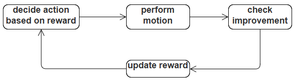
Figure 1. Reward based mechanism
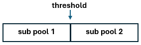
Figure 2. Threshold of RGSO-1
The existence of the random number and reward-based threshold keep the stochastic aspect of the proposed method. It also differentiates this model with the common q-learning model where the decision making tends to be deterministic based on the current value of the q-table [49]. The formalization of RGSO-1 is provided using (7) to (12) while the pseudocode of RGSO-1 is provided in algorithm 2. The source code for both RGSO-1 and RGSO-2 can be downloaded through this link: https://github.com/purbodaru/reward-based-glider-snake-optimization.
| 
| (7) |
| 
| (8) |
Equation (7) and equation (8) constructs the pools and sub pools. Equation (7) shows that each agent has its own pool where P is a set of pool and p is a pool related to an agent. The cardinality of the set of pools equals to the cardinality of swarm. Equation (8) shows that there are two sub pools for each agent.
| 
| (9) |
| 
| (10) |
Equation (9) and (10) are used for the two possible motions of each agent. Equation (9) shows the action taken based on the stochastic manner based on the reward. There are two values for action  which are 1 and 2 which is determined based on the threshold and a random number. is a uniform random number [0,1]. Equation (10) formalizes the construction of the solution candidate based on the chosen motion where
  is the solution candidate.
| 
| (11) |
| 
| (12) |
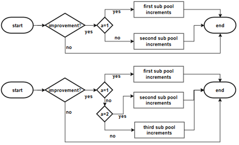
Equation (11) and equation (12) formalize the updating process. Equation (11) formalizes the updating process of the sub pool. Equation (12) formalizes the updating process of the agent using the solution candidate. Both equations are also used for updating the sub pools and the agent in RGSO-2. The flowchart of this updating process can be found in Figure 3.
The complexity analysis of RGSO-1 is as follows. During the initialization, the complexity is  . The common complexity of sorting in the beginning of every iteration is
  . It means that the complexity during iteration will be
  .
.
algorithm 2: RGSO-1 |
1 | begin |
2 | for all |
3 | initialize xi using (3) |
4 | set  to 1 to 1 |
5 | end for |
6 | for to |
7 | = sort() |
8 | for to |
9 | get using (5) and , , and using (4) |
10 | set |
11 | set using (9) |
12 | construct using (10) |
13 | update using (11) |
14 | update using (12) |
15 | end for |
16 | end for |
17 | return |
18 | end |
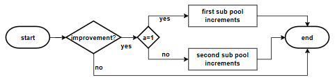
Figure 3. Reward update mechanism of RGSO-1
- Reward Based Glider Snake Optimization (RGSO-2)
RGSO-2 is the second version or the reward-based GSO proposed in this work. RGSO-2 can be seen as an extended version of the RGSO-1. There are two differences between RGSO-2 and RGSO-1. First, there are three motions in RGSO-2. Two motions are same as in GSO and RGSO-1. The third motion is the motion of the best agent away from the related agent. This motion is adopted from the second motion which is the replacement of the lower quality agent. But, as there is no swarm split in both RGSO-1 and RGSO-2, the best agent is selected as replacement because it is the most possible option to replace any agents in the swarm. The movement away from the agent is inspired by the motion in the third iteration window or in the second half of swarm in the second iteration window in MPA [26]. Second, the best agent is transformed from the best agent in the current iteration to the best agent until the current iteration. It is because the value of the best agent is updated each time after a motion is taken by any agent. This best solution update mechanism is also found in BPBO [17].
The consequence of the additional motion is that there are three sub pools for every agent now. The third pool is created to store the reward for the third motion. The additional consequence is there are two thresholds now. The first threshold separates the first sub pool and the second sub pool. The second threshold separates the second sub pool and the third sub pool. The first threshold is obtained by the dividing the reward in the first sub pool with the accumulation reward from all sub pools. The second threshold is obtained by dividing the accumulation of reward from the first and second sub pools with the accumulation of the reward from all sub pools. The visualization of these thresholds is provided in Figure 4. The formalization of RGSO-2 is provided in (13) to (16) while the pseudocode is presented in algorithm 3.
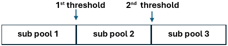
Figure 4. Threshold of RGSO-2
The explanation of (13) to (16) is as follows. Equation (13) declares the pool of every agent consists of three sub pools. Equation (14) shows that the decision of the action based on the stochastic process using two thresholds and there are three possible actions now. Equation (15) shows the construction of the solution candidate based on three possible motions. Equation (16) states the updating of the best agent is based on quality comparison between the best agent and the related agent. Moreover, the reward update mechanism of RGSO-2 is illustrated using Figure 5. As presented in algorithm 2, the complexity of RGSO-2 is equal to RGSO-1. It means that the complexity during initialization is . Meanwhile, the complexity during iteration is .
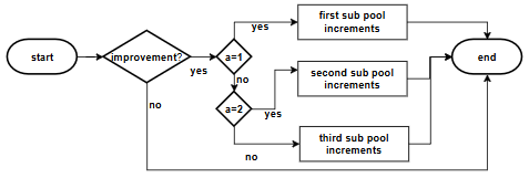
Figure 5. Reward update mechanism of RGSO-2
algorithm 3: RGSO-2 |
1 | begin |
2 | for all |
3 | initialize using (3) |
4 | Update using (16) |
5 | end for |
6 | for to |
7 | = sort() |
8 | for to |
9 | get , , and using (4) |
10 | set |
11 | set using (14) |
12 | construct using (15) |
13 | update using (11) |
14 | update using (12) |
16 | update using (16) |
17 | end for |
18 | end for |
19 | return |
20 | end |
- Economic Load Dispatch Problem
Please fill this section with a system block diagram, research flow diagram, control system block diagram or other that illustrates the research. This section also can be fill with a flowchart or pseudocode of the program. ELDP is a practical optimization problem in electrical engineering, specifically in power system. It is categorized as the continuous one. As practical problem, it has constraints. ELDP becomes very popular optimization problem due to its richness in variants, considerations, and use cases. In general, the system consists of a set of generating units. Each generating unit produces power within its specified range. The power produced by each generating unit is then accumulated to become total power where this total power should meet i.e. equals to the specified demand. Cost is generated as consequence of producing power. Each cost from all generating units is then accumulated to become the total cost. In its standard form, the objective of the problem is to minimize the total cost. Meanwhile, there are two constraints. The first constraint is the power limitation of each generating unit as should be within its range. The second constraint is the equality of total power to the demand. This second constraint makes the power of each generating unit cannot be freely put anywhere within its range as the power of one generating unit affects the power of other generating units. The formalization of ELDP is provided in (17) to (21).
Below is the explanation of (17) to (21). (17) states the system as a set of generating units where  is set of generating units
  with the number of units n. (18) states the power of each generating unit should be within its range of its minimum power
  and maximum power
  . Equation (19) states that the total power should equals to the demand
  . Equation (20) declares the objective
  on minimizing the total cost. Equation (21) formalizes the cost function of each generating unit with two scenarios including without valve point loading effect (NVPLE) or with valve point loading effect (VPLE) where ,
  ,
,  ,
,  , and
, and  are the cost constants.
In this work, round robin-based adjustment is used to handle the equality constraint rather than penalty-based constraint handling. In this round robin-based adjustment, rotating mechanism is applied with small fraction of power for adjustment. If the total power surpasses the demand, then this rotating mechanism is applied to reduce the power of all generating units. This power reduction is applied to the generating units where its power is still above its minimum power. On the other hand, if the total power is below the demand, then this rotating mechanism is applied to increase the power of all generating units. The power increase is applied to the generating units where its power is still below its maximum power. The rotation runs until the total power equals to the demand.
RESULT AND DISCUSSION
Experiment Result
This section provides the experiment and analysis regarding the performance of both RGSO-1 and RGSO-2. Both algorithms are implemented two problems. The first problem is the set of 23 classic functions. The second problem is ELDP. There are three cases for the ELDP including 3-unit system, 5-unit system, and 10-unit system. There are two scenarios for each case of ELDP including NVPLE and VPLE. In this experiment, five existing algorithms are chosen as competitors including GWO [12], HO [13], BPBO [17], GSO [41], and PSO [14]. PSO is chosen as it is a classic and highly cited algorithm. GWO is a relatively new and highly cited algorithm. Both PSO and GWO have numerous variants. BPBO and HO are chosen as new algorithms. GSO is chosen for comparison as both RGSO-1 and RGSO-2 are derivatives of it. There are 30 independent runs for each function or case. The parameter setting for these algorithms is found in Table 1. The maximum iteration is set to 100 for 23 functions and 200 for ELDP. Both values represent moderate computational process.
Table 1. Parameter Setting for Experiment
Algorithm | Parameter |
GWO | 
|
HO |
|
BPBO |
|
GSO | ,  |
PSO | ,  , ,  , ,  |
RGSO-1 |
|
RGSO-2 |
|
This parameter setup is like many existing studies. For example, in [50], the swarm size is 10, the maximum iteration is 200, and the dimension size ranges from 10 to 20. In [46], the swarm size is 25 and the maximum iteration is 100. In [44], the swarm size is 25 and the maximum iteration is 500. In [51], the swarm size is 50 and the maximum iteration is 200. In [21], the swarm size is 30 while the maximum iteration is 500. In [27], as there are also sensitivity analysis to conduct the influence of swarm size and maximum iteration, there are multiple values of swarm size and maximum iteration where the values of swarm size are 30, 50, 80, and 1000 while the values of maximum iteration are 100, 300, 500, and 1000.
The first problem is the set of 23 functions. It can be split into three groups including seven high dimension unimodal functions (HDUF), six high dimension multimodal functions (HDMF), and ten fixed dimension multimodal functions (FDMF). The detail description regarding the 23 functions can be found in [52]. The dimension size for the high dimension functions is 30.
Table 2 exhibits the result for the HDUF. The GSO is slightly superior as it is the best in five functions including F1, F2, F3, F5, and F7. RGSO-2 follows as the second best as it is the best in four functions including F2, F5, F6, and F7. BPBO also achieves the best result in three functions including RGSO-2 achieves the best result in three functions including F2, F4, and F5. All algorithms achieve the best result in F2. PSO becomes the worst algorithm while HO becomes the second worst algorithm.
Table 3 shows the superiority of RGSO-2. It achieves the best result in four functions including F9, F11, F12, and F13. RGSO-1 achieves the best result in F8 and F11. Both GSO and BPBO achieves one best result. PSO becomes the worst algorithm, and HO follows as the second worst.
Table 2. Result for HDUF
F | Parameter | GWO | HO | BPBO | GSO | PSO | RGSO-1 | RGSO-2 |
1 | mean | 0.187 | 2.100× | 9.634x10⁻¹⁵ | 1.714x10-82 | 5.365x10³ | 2.121x10-44 | 4.287x10-38 |
std. deviation | 0.650 | 1.366× | 3.415x10⁻¹⁴ | 9.230x10-82 | 1.889x10³ | 1.140x10-43 | 2.308x10-37 |
mean rank | 5 | 6 | 4 | 1 | 7 | 2 | 3 |
2 | mean | 0.000 | 0.000 | 0.000 | 0.000 | 0.000 | 0.000 | 0.000 |
std. deviation | 0.000 | 0.000 | 0.000 | 0.000 | 0.000 | 0.000 | 0.000 |
mean rank | 1 | 1 | 1 | 1 | 1 | 1 | 1 |
3 | mean | 7.964× | 2.237x10² | 1.279x10⁻⁵ | 2.546x10-71 | 1.763x10⁴ | 1.904x10-37 | 1.628x10-37 |
std. deviation | 4.278× | 1.607x10² | 2.081x10⁻⁵ | 1.350x10-70 | 7.056x10³ | 1.025x10-36 | 8.767x10-37 |
mean rank | 5 | 6 | 4 | 1 | 7 | 3 | 2 |
4 | mean | 0.037 | 2.131 | 1.028x10⁻⁷ | 4.974x10⁻⁵ | 2.772x101 | 1.426x10⁻⁴ | 1.681x10⁻⁵ |
std. deviation | 0.094 | 0.566 | 9.473x10⁻⁸ | 1.114x10⁻⁴ | 5.462 | 3.083x10⁻⁴ | 6.616x10⁻⁵ |
mean rank | 5 | 6 | 1 | 3 | 7 | 4 | 2 |
5 | mean | 1.306x10⁵ | 1.028x10⁴ | 2.889x101 | 2.871x101 | 2.018x10⁶ | 2.871x101 | 2.871x101 |
std. deviation | 7.139x10⁵ | 1.271x10⁴ | 0.060 | 0.001 | 1.234x10⁶ | 4.244x10⁻⁴ | 7.571x10⁻⁴ |
mean rank | 6 | 5 | 4 | 1 | 7 | 1 | 1 |
6 | mean | 7.376 | 4.050x101 | 5.165 | 0.005 | 5.291x10³ | 0.002 | 4.971x10⁻⁴ |
std. deviation | 0.469 | 2.036x101 | 0.410 | 0.008 | 1.398x10³ | 0.003 | 1.474x10⁻³ |
mean rank | 5 | 6 | 4 | 3 | 7 | 2 | 1 |
7 | mean | 0.039 | 9.376x101 | 0.001 | 0.001 | 1.195 | 0.002 | 0.001 |
std. deviation | 0.037 | 4.976x101 | 0.001 | 0.001 | 0.783 | 0.002 | 0.001 |
mean rank | 5 | 7 | 1 | 1 | 6 | 4 | 1 |
Table 3. Result for HDMF
F | Parameter | GWO | HO | BPBO | GSO | PSO | RGSO-1 | RGSO-2 |
8 | mean | -0.442 | -1.025× | -4.048× | -9.778× | -2.723× | -1.041× | -9.570× |
std. deviation | 2.017 | 4.462 | 7.272× | 2.061× | 4.649× | 1.926× | 1.769× |
mean rank | 7 | 6 | 4 | 2 | 5 | 1 | 3 |
9 | mean | 0.738 | 2.998× | 1.515× | 0.003 | 2.355× | 5.455× | 0.000 |
std. deviation | 3.535 | 1.828× | 8.162× | 0.012 | 1.930× | 2.937× | 0.000 |
mean rank | 5 | 7 | 2 | 4 | 6 | 3 | 1 |
10 | mean | 0.008 | 4.432 | 8.342× | 2.985x10⁻⁴ | 1.249× | 5.938× | 4.817× |
std. deviation | 0.025 | 0.760 | 2.859× | 4.750x10⁻⁴ | 1.068 | 9.371× | 1.053× |
mean rank | 5 | 6 | 1 | 4 | 7 | 3 | 2 |
11 | mean | 0.076 | 0.260 | 4.694× | 0.000 | 5.318× | 0.000 | 0.000 |
std. deviation | 0.409 | 0.178 | 0.002 | 0.000 | 1.598× | 0.000 | 0.000 |
mean rank | 5 | 6 | 4 | 1 | 7 | 1 | 1 |
12 | mean | 1.704 | 3.230 | 0.658 | 0.001 | 7.783× | 2.531× | 5.714× |
std. deviation | 0.244 | 0.759 | 0.146 | 0.001 | 2.150× | 2.951× | 9.307× |
mean rank | 5 | 6 | 4 | 3 | 7 | 2 | 1 |
13 | mean | 3.182 | 2.860 | 2.825 | 4.793× | 2.155× | 8.197× | 6.373× |
std. deviation | 0.195 | 1.445 | 0.191 | 1.100× | 1.954× | 1.204× | 1.137× |
mean rank | 6 | 5 | 4 | 3 | 7 | 2 | 1 |
Table 4 shows the continuous superiority of RGSO-2. RGSO-2 achieves the best result in seven functions including F16, F17, and F19-F23. BPBO stays as the second best as it achieves the best result in four functions including F14, F15, F17, and F19. GSO achieves the best result in three functions including F16, F17, and F19. GWO becomes the worst algorithm followed by HO as the second worst.
Table 5 and Table 6 exhibits the Wilcoxon rank test to compare the difference between the proposed algorithms and competitors as non-parametrical statistical test. There are several reasons on using Wilcoxon test rather than other tests such as t-test or Friedman test. First, the normality of the data distribution cannot be guaranteed as it is the requirement of conducting the t-test. Second, the Wilcoxon test is suiter in comparing two sets of data while Friedman test is suiter in comparing multiple sets of data. In this context, the comparison analysis is conducted to investigate the difference of the proposed RGSO with each of the benchmark algorithms. Third, the Wilcoxon test is more common as non-parametrical statistical test for many studies introducing new algorithms, such as in GAO [22], POA [23], COA [19], and so on. Table 5 shows the result for comparison of RGSO-1 with other algorithms while Table 6 for comparison of RGSO-2 with other algorithms. The 0.05 threshold is used. There are two values including SD for significantly different and NSD for not significantly different. Table 5 shows that the number of functions which are significantly different to RGSO-1 is 2, 1, 5, 14, 4, and 10 consecutively for GWO, HO, BPBO, GSO, PSO, and RGSO-2. On the other hand, Table 6 shows that the number of functions which are significantly different to RGSO-2 is 1, 1, 8, 11, 1, and 10 consecutively to GWO, HO, BPBO, GSO, PSO, and RGSO-1.
Table 4. Result for FDMF
F | Parameter | GWO | HO | BPBO | GSO | PSO | RGSO-1 | RGSO-2 |
14 | mean | 1.267× | 1.267× | 5.046 | 7.427 | 5.095 | 8.944 | 8.189 |
std. deviation | 0.000 | 0.013 | 3.930 | 4.780 | 3.324 | 5.114 | 5.065 |
mean rank | 6 | 6 | 1 | 3 | 2 | 5 | 4 |
15 | mean | 0.148 | 0.037 | 5.470× | 0.004 | 0.027 | 0.001 | 5.577× |
std. deviation | 0.000 | 0.051 | 2.417× | 0.017 | 0.034 | 5.975x× | 4.376× |
mean rank | 7 | 6 | 1 | 4 | 5 | 3 | 2 |
16 | mean | 0.000 | -0.536 | -1.028 | -1.031 | -1.004 | -1.022 | -1.031 |
std. deviation | 0.000 | 0.342 | 0.004 | 6.739× | 0.131 | 0.034 | 9.408× |
mean rank | 7 | 6 | 3 | 1 | 5 | 4 | 1 |
17 | mean | 5.562× | 0.839 | 0.398 | 0.398 | 0.526 | 0.408 | 0.398 |
std. deviation | 0.146 | 0.440 | 1.291× | 2.012× | 0.285 | 0.055 | 6.807× |
mean rank | 7 | 6 | 1 | 1 | 5 | 4 | 1 |
18 | mean | 6.000× | 9.640× | 4.304 | 8.432 | 4.175 | 7.565 | 6.793 |
std. deviation | 0.000 | 1.167× | 5.183 | 2.032× | 4.985 | 1.021× | 9.680 |
mean rank | 6 | 5 | 2 | 4 | 1 |
| 3 |
19 | mean | -0.001 | -0.048 | -0.049 | -0.049 | -0.001 | -0.049 | -0.049 |
std. deviation | 0.004 | 0.004 | 0.000 | 0.000 | 0.002 | 0.000 | 0.000 |
mean rank | 6 | 5 | 1 | 1 | 6 | 1 | 1 |
20 | mean | -0.005 | -1.087 | -2.905 | -2.377 | -2.392 | -2.537 | -2.959 |
std. deviation | 0.000 | 0.663 | 0.230 | 0.633 | 0.564 | 0.532 | 0.388 |
mean rank | 7 | 6 | 2 | 5 | 4 | 3 | 1 |
21 | mean | -0.273 | -1.234 | -5.544 | -1.011× | -4.216 | -1.014× | -1.015× |
std. deviation | 0.000 | 0.832 | 2.297 | 0.050 | 2.842 | 0.015 | 0.006 |
mean rank | 7 | 6 | 4 | 3 | 5 | 2 | 1 |
22 | mean | -0.293 | -1.668 | -6.122 | -1.037× | -4.984 | -1.038× | -1.040× |
std. deviation | 0.000 | 0.840 | 2.402 | 0.075 | 3.051 | 0.037 | 0.004 |
mean rank | 7 | 6 | 4 | 3 | 5 | 2 | 1 |
23 | mean | -0.321 | -1.463 | -5.298 | -1.052x101 | -4.499 | -1.052× | -1.053× |
std. deviation | 0.000 | 0.391 | 2.268 | 0.031 | 2.616 | 0.028 | 0.004 |
mean rank | 7 | 6 | 4 | 2 | 5 | 2 | 1 |
Table 5. Wilcoxon Rank Test for Comparison between RGSO-1 and Its Benchmarks
F | GWO | HO | BPBO | GSO | PSO | RGSO-2 |
1 | SD | SD | SD | SD | SD | NSD |
2 | NSD | SD | NSD | NSD | NSD | NSD |
3 | SD | SD | SD | SD | SD | NSD |
4 | SD | SD | SD | NSD | SD | SD |
5 | SD | SD | SD | SD | SD | SD |
6 | SD | SD | SD | SD | SD | SD |
7 | SD | SD | SD | NSD | SD | SD |
8 | SD | SD | SD | NSD | SD | NSD |
9 | SD | SD | NSD | SD | SD | NSD |
10 | NSD | SD | SD | NSD | SD | SD |
11 | SD | SD | SD | NSD | SD | NSD |
12 | SD | SD | SD | SD | SD | SD |
13 | SD | SD | SD | NSD | SD | NSD |
14 | SD | SD | SD | NSD | SD | NSD |
15 | SD | SD | SD | NSD | SD | SD |
16 | SD | SD | NSD | SD | NSD | SD |
17 | SD | SD | NSD | NSD | SD | SD |
18 | SD | SD | SD | NSD | NSD | NSD |
19 | SD | NSD | NSD | NSD | SD | NSD |
20 | SD | SD | SD | NSD | NSD | SD |
21 | SD | SD | SD | SD | SD | SD |
22 | SD | SD | SD | NSD | SD | SD |
23 | SD | SD | SD | SD | SD | SD |
Total NSD | 2 | 1 | 5 | 14 | 4 | 10 |
Total SD | 21 | 22 | 18 | 9 | 19 | 13 |
Table 6. Wilcoxon Rank Test for Comparison between RGSO-2 and Its Benchmarks
F | GWO | HO | BPBO | GSO | PSO | RGSO-1 |
1 | SD | SD | SD | SD | SD | NSD |
2 | NSD | SD | NSD | NSD | NSD | NSD |
3 | SD | SD | SD | SD | SD | NSD |
4 | SD | SD | SD | NSD | SD | SD |
5 | SD | SD | SD | NSD | SD | SD |
6 | SD | SD | SD | SD | SD | SD |
7 | SD | SD | SD | SD | SD | SD |
8 | SD | SD | SD | NSD | SD | NSD |
9 | SD | SD | NSD | SD | SD | NSD |
10 | SD | SD | NSD | SD | SD | SD |
11 | SD | SD | SD | NSD | SD | NSD |
12 | SD | SD | SD | SD | SD | SD |
13 | SD | SD | SD | NSD | SD | NSD |
14 | SD | SD | NSD | NSD | SD | NSD |
15 | SD | SD | NSD | NSD | SD | SD |
16 | SD | SD | SD | SD | SD | SD |
17 | SD | SD | SD | SD | SD | SD |
18 | SD | SD | NSD | NSD | SD | NSD |
19 | SD | NSD | NSD | NSD | SD | NSD |
20 | SD | SD | NSD | SD | SD | SD |
21 | SD | SD | SD | SD | SD | SD |
22 | SD | SD | SD | SD | SD | SD |
23 | SD | SD | SD | NSD | SD | SD |
Total NSD | 1 | 1 | 8 | 11 | 1 | 10 |
Total SD | 22 | 22 | 15 | 12 | 22 | 13 |
Table 7 reports the sensitivity analysis regarding the different values of swarm size. As mentioned previously, the increase of maximum iteration is not considered as this issue has been covered in the convergence analysis as reported in Figures 6. Meanwhile, the various values of threshold are not carried out as the RGSO is designed to provide equal size of sub pools. Moreover, violating the equal size sub pools provides abundance of combinations regarding the threshold in RGSO-1 and two thresholds in RGSO-2. There are two values for each RGSO including 25 and 50. The result shows that significant improvements occur only in five functions for RGSO-1 and nine functions for RGSO-2. All these five functions for RGSO-1 are high dimension functions while eight of nine functions for RGSO-2 are high dimension functions. It means that the increase of swarm size above 20 does not affect significantly for fixed dimension functions in general.
Table 7. Sensitivity Analysis based on Swarm Size
F | RGSO-1 | RGSO-2 |
n=25 | n=50 | Significant improvement | n=25 | n=50 | Significant improvement |
1 | 2.259× | 2.257× | yes | 5.534× | 2.198× | yes |
2 | 0.000 | 0.000 | no | 0.000 | 0.000 | no |
3 | 1.149× | 1.653× | no | 6.418× | 2.518× | yes |
4 | 1.184× | 3.806× | yes | 3.404× | 2.535× | yes |
5 | 2.871× | 2.871× | no | 2.871× | 2.871× | no |
6 | 0.001 | 4.047× | yes | 1.071× | 1.371× | yes |
7 | 0.001 | 7.116× | no | 0.001 | 2.391× | yes |
8 | -1.073× | -1.224× | yes | -1.044× | -1.116× | no |
9 | 0.000 | 0.000 | no | 5.684× | 0.000 | yes |
10 | 2.253× | 5.138× | yes | 2.137× | 6.297× | yes |
11 | 0.000 | 0.000 | no | 0.000 | 0.000 | no |
12 | 1.097× | 1.262× | no | 6.405× | 3.649× | no |
13 | 4.189× | 2.217× | no | 7.944× | 3.901× | yes |
14 | 8.258 | 4.398 | no | 7.757 | 4.360 | no |
15 | 9.033× | 5.255× | no | 5.066× | 5.270× | no |
16 | -1.030 | -1.031 | no | -1.031 | -1.031 | no |
17 | 0.398 | 0.398 | no | 0.398 | 0.398 | no |
18 | 6.610 | 5.700 | no | 1.300× | 3.900 | yes |
19 | -0.049 | -0.049 | no | -0.049 | -0.049 | no |
20 | -2.657 | -2.875 | no | -2.913 | -3.055 | no |
21 | -1.014× | -1.015× | no | -1.015× | -1.015× | no |
22 | -1.038× | -1.039× | no | -1.040× | -1.040× | no |
23 | -1.052× | -1.053× | no | -1.053× | -1.053× | no |
Figure 6 shows the convergence analysis on solving the 23 functions. There are three samples for the iteration including 1, 50, and 100. They represent the first iteration, half of maximum iteration, and the maximum iteration. The result shows that both RGSO-1 and RGSO-2 converge in the half of the maximum iteration in all functions. This convergence behaviour is also found in other benchmark algorithms except GWO in some functions. Based on this circumstance, there is no need to conduct additional test for higher maximum iteration.
Figure 6. Convergence analysis of 23 functions
The first case in the second problem is 3-unit system. The system consists of three generating units. The demand is 850 MW. The detail description of this system can be found in [53]. The result is exhibited in Table 8 for NVPLE and Table 9 for VPLE. Table 8 shows that five algorithms including BPBO, GSO, PSO, RGSO-1, and RGSO-2 performs equally while GWO becomes the worst algorithm. Meanwhile, Table 9 shows that BPBO becomes the best algorithm in VPLE. The performance of GSO, RGSO-1, and RGSO-2 is almost equal. GWO still becomes the worst algorithm.
The second case is the 5-unit system. The system consists of five generating units. The detail description of this system can be found in [53]. The demand is 730 MW. The result is exhibited in Table 10 for NVPLE and Table 11 for VPLE. Table 10 shows that RGSO-2 becomes the best algorithm while RGSO-1, GSO, and BPBO follow in the second place for NVPLE. The difference between RGSO-2 and these three algorithms is very narrow. GWO becomes the worst followed by HO in the second worst. In the VPLE, BPBO becomes the best while RGSO-2 becomes the second best and RGSO-1 becomes the third best. The difference between RGSO-2 and RGSO-1 is very narrow. GWO still becomes the worst followed by HO as the second worst.
The third case is 10-unit system. This system consists of ten generating units. The detail description of this system can be found in [54]. The demand is 2,000 MW. The result is provided in Table 12 for NVPLE and Table 13 for VPLE. Table 12 exhibits that RGSO-2 becomes the best algorithm followed by GSO in the second place for NVPLE. Table 13 exhibits that GSO becomes the best algorithm followed by RGSO-2 as the second best. Meanwhile, the difference among four algorithms including BPBO, GSO, RGSO-1, and RGSO-2 is narrow for both scenarios. In both scenarios, GWO becomes the worst followed by HO as the second worst.
Table 8. Result for ELDP on 3-unit System without VPLE
Parameter | GWO | HO | BPBO | GSO | PSO | RGSO-1 | RGSO-2 |
avg.  (MW) (MW) | 439.7 | 387.3 | 393.3 | 393.1 | 393.5 | 393.1 | 393.0 |
avg.  (MW) (MW) | 266.4 | 339.0 | 334.7 | 334.9 | 334.0 | 334.9 | 335.0 |
avg.  (MW) (MW) | 143.9 | 123.7 | 122.0 | 122.0 | 122.5 | 122.0 | 122.0 |
avg. total cost ($) | 8,237.2 | 8,196.6 | 8,194.3 | 8,194.3 | 8,194.3 | 8,194.3 | 8,194.3 |
rank | 7 | 6 | 1 | 1 | 1 | 1 | 1 |
Table 9. Result for ELDP on 3-unit System with VPLE
Parameter | GWO | HO | BPBO | GSO | PSO | RGSO-1 | RGSO-2 |
avg. (MW) | 432.3 | 397.1 | 366.4 | 373.3 | 439.5 | 387.0 | 387.1 |
avg. (MW) | 277.6 | 260.6 | 350.3 | 330.0 | 277.2 | 279.0 | 283.8 |
avg. (MW) | 140.1 | 192.3 | 133.3 | 146.7 | 133.3 | 184.0 | 179.1 |
avg. total cost ($) | 8,644.4 | 8,296.7 | 8,236.8 | 8,244.7 | 8,307.4 | 8,248.0 | 8,248.3 |
rank | 7 | 5 | 1 | 2 | 6 | 3 | 4 |
Table 10. Result for ELDP on 5-unit System without VPLE
Parameter | GWO | HO | BPBO | GSO | PSO | RGSO-1 | RGSO-2 |
(MW) | 227.2 | 225.8 | 223.8 | 223.9 | 237.5 | 222.6 | 222.3 |
(MW) | 106.5 | 97.4 | 95.6 | 95.0 | 94.7 | 94.9 | 95.0 |
(MW) | 140.5 | 142.2 | 152.4 | 151.4 | 143.5 | 151.9 | 151.9 |
 (MW) (MW)
| 60.8 | 47.7 | 28.7 | 29.2 | 36.4 | 28.9 | 29.0 |
 (MW) (MW)
| 195.0 | 216.9 | 229.5 | 230.5 | 217.9 | 231.7 | 231.8 |
total cost ($) | 1,968.1 | 1,957.5 | 1,950.6 | 1,950.6 | 1,952.3 | 1,950.6 | 1,950.5 |
rank | 7 | 6 | 2 | 2 | 5 | 2 | 1 |
Table 11. Result for ELDP on 5-unit System with VPLE
Parameter | GWO | HO | BPBO | GSO | PSO | RGSO-1 | RGSO-2 |
(MW) | 233.3 | 229.4 | 234.0 | 218.1 | 230.3 | 227.2 | 230.9 |
(MW) | 105.4 | 112.2 | 100.6 | 112.4 | 103.0 | 112.0 | 111.8 |
(MW) | 146.9 | 131.5 | 118.6 | 140.7 | 122.9 | 138.1 | 136.5 |
(MW) | 62.1 | 72.2 | 66.9 | 73.8 | 61.6 | 73.0 | 65.9 |
(MW) | 182.3 | 184.7 | 209.9 | 185.0 | 212.2 | 179.7 | 184.9 |
total cost ($) | 2,473.9 | 2,273.8 | 2,072.6 | 2,152.1 | 2,165.1 | 2,147.5 | 2,147.4 |
rank | 7 | 6 | 1 | 4 | 5 | 3 | 2 |
Table 12. Result for ELDP on 10-unit System without VPLE
Parameter | GWO | HO | BPBO | GSO | PSO | RGSO-1 | RGSO-2 |
(MW) | 49.6 | 53.6 | 53.0 | 54.6 | 51.7 | 54.6 | 55.0 |
(MW) | 72.3 | 77.7 | 77.7 | 79.2 | 76.2 | 79.6 | 79.8 |
(MW) | 110.2 | 114.7 | 91.4 | 93.3 | 111.6 | 96.1 | 85.9 |
(MW) | 121.5 | 114.2 | 80.8 | 77.7 | 113.0 | 77.0 | 75.1 |
(MW) | 144.7 | 137.9 | 66.3 | 63.2 | 122.0 | 63.3 | 63.1 |
 (MW) (MW)
| 216.5 | 144.6 | 74.8 | 70.0 | 146.1 | 70.0 | 70.0 |
 (MW) (MW)
| 261.9 | 252.0 | 292.0 | 290.5 | 246.7 | 288.9 | 295.3 |
 (MW) (MW)
| 275.6 | 288.5 | 329.5 | 331.6 | 280.5 | 330.7 | 336.0 |
 (MW) (MW)
| 376.1 | 427.0 | 466.8 | 470.0 | 421.8 | 469.9 | 469.9 |
 (MW) (MW)
| 371.6 | 389.8 | 467.7 | 469.9 | 430.4 | 469.9 | 469.9 |
total cost ($) | 111,293.4 | 108,729.6 | 106,026.0 | 105,996.7 | 108,261.4 | 106,003.4 | 105,977.5 |
rank | 7 | 6 | 4 | 2 | 5 | 3 | 1 |
Table 13. Result for ELDP on 10-unit System with VPLE
Parameter | GWO | HO | BPBO | GSO | PSO | RGSO-1 | RGSO-2 |
(MW) | 49.5 | 53.3 | 53.5 | 54.8 | 52.2 | 54.6 | 54.9 |
(MW) | 74.6 | 78.3 | 77.7 | 79.2 | 76.6 | 79.5 | 79.7 |
(MW) | 111.9 | 115.6 | 90.4 | 91.5 | 112.3 | 93.9 | 87.3 |
(MW) | 124.3 | 112.9 | 82.2 | 76.8 | 116.4 | 76.8 | 75.3 |
(MW) | 148.6 | 137.3 | 66.1 | 63.0 | 119.2 | 63.3 | 61.5 |
(MW) | 218.8 | 149.5 | 75.4 | 70.1 | 146.4 | 70.1 | 70.0 |
(MW) | 257.7 | 249.2 | 291.5 | 291.4 | 247.4 | 290.0 | 294.8 |
(MW) | 281.7 | 301.1 | 328.9 | 333.3 | 283.5 | 331.9 | 336.5 |
(MW) | 364.4 | 400.1 | 467.0 | 469.9 | 415.3 | 469.9 | 470.0 |
(MW) | 368.5 | 402.7 | 467.3 | 470.0 | 430.7 | 470.0 | 470.0 |
total cost ($) | 111,819.6 | 109,107.9 | 106,236.0 | 106,191.2 | 108,454.2 | 106,207.6 | 106,200.1 |
rank | 7 | 6 | 4 | 1 | 5 | 3 | 2 |
Discussion
In general, the experiment results show that both RGSO-1 and RGSO-2 are competitive in handling both set of problems. Both RGSO-1 and RGSO-2 are superior compared to three algorithms including GWO, HO, and PSO. The result also shows that RGSO-2 tends to be the best algorithm which means that RGSO-2 is better than RGSO-1. The performance of RGSO-1 is comparable to GSO as its origin and BPBO.
Overall, these seven algorithms can be split into two clusters based on their performance. The first cluster consists of RGSO-1, RGSO-2, BPBO, and GSO. The second cluster consists of GWO, HO, and PSO. The performance of algorithms in the first cluster is better than algorithms in the second cluster. As algorithms in the first cluster conduct multiple strategy approach while algorithms in the second cluster conduct single strategy approach, it can be said that algorithms with multiple strategies tend to perform better than algorithms with single strategy.
By comparing RGSO-1 and RGSO-2, adding the third search, which is the motion toward the best agent where the best agent is updated each time the motion is conducted provides significant improvement. RGSO-2 is better than RGSO-1 in many functions of 23 functions and many cases in ELDP. RGSO-1 outperforms RGSO-2 only in F1, F8, and 3-unit system with VPLE. As, the third motion tends to be more focus on the best agent, it can be said that adding more portion for the best agent-oriented search produces better performance than managing equal probability between both searches as it is found in RGSO-1.
This statement is strengthened by comparing RGSO-1 and GSO. Based on the model, GSO provides 75 percent probability for best-agent oriented search and 25 percent probability for random agent-oriented search. Meanwhile, RGSO-1 provides equal probability between both searches. Based on the result on solving 23 functions, GSO is slightly better than RGSO-1 in the HDUF while RGSO-1 is slightly better than GSO in HDMF and FDMF. Meanwhile, RGSO-1 and GSO are almost equal in ELDP.
There are limitations regarding the proposed RGSO in specific and the work in general. First, this is a modification of existing GSO. Meanwhile, there are also various modifications that can be conducted. Second, this modification, which is the reward-based mechanism is applied to GSO. On the other hand, there are abundance metaheuristic algorithms that perform multiple search strategy where this reward-based mechanism can also be applied to them. Third, the experiments are limited to the 23 functions and three systems for ELDP. This single paper cannot cover broader benchmark cases such as CEC series, more various case of ELDP, and broader practical engineering problems as excessive paper length becomes the consequence. The excessive paper length in one research paper where the experiment dominates the paper makes the scientific contributions and novelties seem less significant.
CONCLUSIONS
In this study, we have proposed two modified versions of the existing GSO using reward-based approach which is adopted from the RL called as RGSO-1 and RGSO-2. The experiment results show that RGSO-2 is superior in almost all functions compared to RGSO-1 and GSO. Meanwhile, the performance of RGSO-1 is comparable to GSO which means that RGSO-1 is better than GSO in some problems but worse than GSO in other problems. RGSO-1 is better than GSO in multimodal functions while GSO is better than RGSO-1 in unimodal functions. The result also shows that algorithms with multiple search strategy are better than algorithms with single search strategy as BPBO, GSO, RGSO-1, and RGSO-2 tend to be better than GWO, HO, and PSO. Moreover, through comparing RGSO-1 and RGSO-2, allocating more portion for best-agent oriented search than random agent-oriented search is better than allocating equal portion for both searches. Meanwhile, the limitations of both RGSOs are that their performance is still comparable with the standard GSO and BPBO. Moreover, as referred to the NFL theory, both RGSO-1 and RGSO-2 are not superior to solve all problems.
There are several trajectories can be taken for future studies. First, as this reward-based mechanism is applied only in GSO, this mechanism can also be applied in many other existing algorithms. More comprehensive investigation is needed to analyse the performance of this mechanism in other algorithms. Second, this reward-based mechanism can also be explored and improved to construct better mechanisms in determining the search strategy rather than the existing probabilistic, sequential, and split mechanisms as there are a lot of RL-based methods that be adopted as RL is suitable for reward-based system. Third, both proposed RGSO-1 and RGSO-2 can be applied to solve broader optimization problems, both the continuous and discrete ones, such as allocation problems, timetabling problems, scheduling problems, routing problems, and so on.
DECLARATION
Sustainable Development Goals
Affordable and Clean Energy (SDG 7) and Industry, Innovation and Infrastructure (SDG 9)
Author Contribution
PBD: conceptualization, modelling, software, data acquisition, writing draft, funding. BI: modelling, formal analysis, writing-review, funding. All authors read and approved the final paper.
Funding
The publication of this work is supported by Telkom University without specific grant.
Conflicts of Interest
The authors declare no conflict of interest.
REFERENCES
- D. C. Secui, G. Bendea, M. L. Secui, C. Hora, and C. Bendea, “The Chaotic Social Group Optimization for the Economic Dispatch Problem,” International Journal of Intelligent Engineering and Systems, vol. 14, no. 6, pp. 666–677, Dec. 2021, https://doi.org/10.22266/ijies2021.1231.59.
- H. M. Rosli, S. A. Halim, L. J. Awalin, and S. M. Mustaza, “Economic-emission load dispatch for power system operation using enhanced sunflower optimization,” Indonesian Journal of Electrical Engineering and Computer Science, vol. 27, no. 1, pp. 1–10, Jul. 2022, https://doi.org/10.11591/ijeecs.v27.i1.pp1-10.
- L. Mbangeni and S. Krishnamurthy, “A Lagrange-Based Multi-Objective Framework for Wind–Thermal Economic Emission Dispatch,” Processes, vol. 13, no. 9, p. 2814, Sep. 2025, https://doi.org/10.3390/pr13092814.
- S. Syama, J. Ramprabhakar, R. Anand, and J. M. Guerrero, “An integrated binary metaheuristic approach in dynamic unit commitment and economic emission dispatch for hybrid energy systems,” Sci. Rep., vol. 14, no. 1, p. 23964, Oct. 2024, https://doi.org/10.1038/s41598-024-75743-0.
- X.-R. Tao, Q.-K. Pan, and L. Gao, “An efficient self-adaptive artificial bee colony algorithm for the distributed resource-constrained hybrid flowshop problem,” Comput. Ind. Eng., vol. 169, p. 108200, Jul. 2022, https://doi.org/10.1016/j.cie.2022.108200.
- L. Cheng, Q. Tang, L. Zhang, and Z. Li, “Inventory and total completion time minimization for assembly job-shop scheduling considering material integrity and assembly sequential constraint,” J. Manuf. Syst., vol. 65, pp. 660–672, Oct. 2022, https://doi.org/10.1016/j.jmsy.2022.10.013.
- J. Xu, W. Hu, W. Gu, and Y. Yu, “A Discrete JAYA Algorithm Based on Reinforcement Learning and Simulated Annealing for the Traveling Salesman Problem,” Mathematics, vol. 11, no. 14, p. 3221, Jul. 2023, https://doi.org/10.3390/math11143221.
- B. Ye et al., “Multi-Depot Vehicle Routing Problem with Collaborative Replenishment Using ALNS–ABC Algorithm,” International Journal of Software Engineering and Knowledge Engineering, vol. 36, no. 04, pp. 567–593, Mar. 2026, https://doi.org/10.1142/S0218194025500834.
- Y. Zheng, W. Gai, J. Zhang, and M. Zhong, “A collaborative bi-level optimization approach for smart logistics: Depot location and unmanned aerial vehicle-based pickup-delivery services,” Eng. Appl. Artif. Intell., vol. 165, p. 113453, Feb. 2026, https://doi.org/10.1016/j.engappai.2025.113453.
- Z. Zhang, L. Zhang, and W. Li, “An improved adaptive variable neighborhood search algorithm for stochastic order allocation problem,” Sci. Rep., vol. 15, no. 1, p. 481, Jan. 2025, https://doi.org/10.1038/s41598-024-84663-y.
- M. Almarashi, W. Deabes, H. H. Amin, and A.-R. Hedar, “Simulated Annealing with Exploratory Sensing for Global Optimization,” Algorithms, vol. 13, no. 9, p. 230, Sep. 2020, https://doi.org/10.3390/a13090230.
- S. Mirjalili, S. M. Mirjalili, and A. Lewis, “Grey Wolf Optimizer,” Advances in Engineering Software, vol. 69, pp. 46–61, Mar. 2014, https://doi.org/10.1016/j.advengsoft.2013.12.007.
- S. O. Oladejo, S. O. Ekwe, and S. Mirjalili, “The Hiking Optimization Algorithm: A novel human-based metaheuristic approach,” Knowl. Based. Syst., vol. 296, no. 5, p. 111880, Jul. 2024, https://doi.org/10.1016/j.knosys.2024.111880.
- A. G. Gad, “Particle Swarm Optimization Algorithm and Its Applications: A Systematic Review,” Archives of Computational Methods in Engineering, vol. 29, no. 5, pp. 2531–2561, Aug. 2022, https://doi.org/10.1007/s11831-021-09694-4.
- S. Katoch, S. S. Chauhan, and V. Kumar, “A review on genetic algorithm: past, present, and future,” Multimed. Tools Appl., vol. 80, no. 5, pp. 8091–8126, Feb. 2021, https://doi.org/10.1007/s11042-020-10139-6.
- A. Kumar, D. Kumar, and S. K. Jarial, “A Review on Artificial Bee Colony Algorithms and Their Applications to Data Clustering,” Cybernetics and Information Technologies, vol. 17, no. 3, pp. 3–28, Sep. 2017, https://doi.org/10.1515/cait-2017-0027.
- M. Ghasemi et al., “Birds of prey-based optimization (BPBO): a metaheuristic algorithm for optimization,” Evol. Intell., vol. 18, no. 4, p. 88, Aug. 2025, https://doi.org/10.1007/s12065-025-01052-8.
- M. Dehghani, Z. Montazeri, E. Trojovská, and P. Trojovský, “Coati Optimization Algorithm: A new bio-inspired metaheuristic algorithm for solving optimization problems,” Knowl. Based. Syst., vol. 259, p. 110011, Jan. 2023, https://doi.org/10.1016/j.knosys.2022.110011.
- H. Jia, H. Rao, C. Wen, and S. Mirjalili, “Crayfish optimization algorithm,” Artif. Intell. Rev., vol. 56, no. S2, pp. 1919–1979, Nov. 2023, https://doi.org/10.1007/s10462-023-10567-4.
- S. Suyanto, A. A. Ariyanto, and A. F. Ariyanto, “Komodo Mlipir Algorithm,” Appl. Soft Comput., vol. 114, pp. 1–17, Jan. 2022, https://doi.org/10.1016/j.asoc.2021.108043.
- S. Mirjalili, “SCA: A Sine Cosine Algorithm for solving optimization problems,” Knowl. Based. Syst., vol. 96, pp. 120–133, Mar. 2016, https://doi.org/10.1016/j.knosys.2015.12.022.
- O. Alsayyed et al., “Giant Armadillo Optimization: A New Bio-Inspired Metaheuristic Algorithm for Solving Optimization Problems,” Biomimetics, vol. 8, no. 8, p. 619, Dec. 2023, https://doi.org/10.3390/biomimetics8080619.
- O. Al-Baik et al., “Pufferfish Optimization Algorithm: A New Bio-Inspired Metaheuristic Algorithm for Solving Optimization Problems,” Biomimetics, vol. 9, no. 2, p. 65, Jan. 2024, https://doi.org/10.3390/biomimetics9020065.
- M. Dehghani, Š. Hubálovský, and P. Trojovský, “A new optimization algorithm based on average and subtraction of the best and worst members of the population for solving various optimization problems,” PeerJ Comput. Sci., vol. 8, pp. 1–40, Mar. 2022, https://doi.org/10.7717/peerj-cs.910.
- P. Trojovský and M. Dehghani, “Subtraction-Average-Based Optimizer: A New Swarm-Inspired Metaheuristic Algorithm for Solving Optimization Problems,” Biomimetics, vol. 8, no. 2, p. 149, Apr. 2023, https://doi.org/10.3390/biomimetics8020149.
- A. Faramarzi, M. Heidarinejad, S. Mirjalili, and A. H. Gandomi, “Marine Predators Algorithm: A nature-inspired metaheuristic,” Expert Syst. Appl., vol. 152, p. 113377, Aug. 2020, https://doi.org/10.1016/j.eswa.2020.113377.
- N. Chopra and M. Mohsin Ansari, “Golden jackal optimization: A novel nature-inspired optimizer for engineering applications,” Expert Syst. Appl., vol. 198, p. 116924, Jul. 2022, https://doi.org/10.1016/j.eswa.2022.116924.
- E. Trojovska, M. Dehghani, and P. Trojovsky, “Zebra Optimization Algorithm: A New Bio-Inspired Optimization Algorithm for Solving Optimization Algorithm,” IEEE Access, vol. 10, pp. 49445–49473, 2022, https://doi.org/10.1109/ACCESS.2022.3172789.
- P. Trojovský and M. Dehghani, “Pelican Optimization Algorithm: A Novel Nature-Inspired Algorithm for Engineering Applications,” Sensors, vol. 22, no. 3, pp. 1–34, Jan. 2022, https://doi.org/10.3390/s22030855.
- J. Wang, W. Wang, X. Hu, L. Qiu, and H. Zang, “Black-winged kite algorithm: a nature-inspired meta-heuristic for solving benchmark functions and engineering problems,” Artif. Intell. Rev., vol. 57, no. 4, p. 98, Mar. 2024, https://doi.org/10.1007/s10462-024-10723-4.
- A. Mohammadzadeh and S. Mirjalili, “Eel and grouper optimizer: a nature-inspired optimization algorithm,” Cluster Comput., vol. 27, no. 9, pp. 12745–12786, Dec. 2024, https://doi.org/10.1007/s10586-024-04545-w.
- A. El Romeh, V. Snášel, and S. Mirjalili, “Dholes-inspired optimization (DIO): a nature-inspired algorithm for engineering optimization problems,” Cluster Comput., vol. 28, no. 13, p. 853, Nov. 2025, https://doi.org/10.1007/s10586-025-05543-2.
- A. Ghiaskar, A. Amiri, and S. Mirjalili, “Polar fox optimization algorithm: a novel meta-heuristic algorithm,” Neural Comput. Appl., vol. 36, no. 33, pp. 20983–21022, Nov. 2024, https://doi.org/10.1007/s00521-024-10346-4.
- T. Sharifi, M. Mirsalim, F. Soleimanian Gharehchopogh, and S. Mirjalili, “Cultural history optimization algorithm: a new human-inspired metaheuristic algorithm for engineering optimization problems,” Neural Comput. Appl., vol. 37, no. 25, pp. 21009–21068, Sep. 2025, https://doi.org/10.1007/s00521-025-11379-z.
- F. Rezaei, H. R. Safavi, M. Abd Elaziz, and S. Mirjalili, “GMO: geometric mean optimizer for solving engineering problems,” Soft comput., vol. 27, no. 15, pp. 10571–10606, Aug. 2023, https://doi.org/10.1007/s00500-023-08202-z.
- M. A. Akbari, M. Zare, R. Azizipanah-abarghooee, S. Mirjalili, and M. Deriche, “The cheetah optimizer: a nature-inspired metaheuristic algorithm for large-scale optimization problems,” Sci. Rep., vol. 12, no. 1, p. 10953, Jun. 2022, https://doi.org/10.1038/s41598-022-14338-z.
- M. Ghasemi, M. Zare, A. Zahedi, M.-A. Akbari, S. Mirjalili, and L. Abualigah, “Geyser Inspired Algorithm: A New Geological-inspired Meta-heuristic for Real-parameter and Constrained Engineering Optimization,” J. Bionic Eng., vol. 21, no. 1, pp. 374–408, Jan. 2024, https://doi.org/10.1007/s42235-023-00437-8.
- E. Trojovska and M. Dehghani, “Clouded Leopard Optimization: A New Nature-Inspired Optimization Algorithm,” IEEE Access, vol. 10, pp. 102876–102906, 2022, https://doi.org/10.1109/ACCESS.2022.3208700.
- M. Dehghani and P. Trojovský, “Osprey optimization algorithm: A new bio-inspired metaheuristic algorithm for solving engineering optimization problems,” Front. Mech. Eng., vol. 8, p. 1126450, Jan. 2023, https://doi.org/10.3389/fmech.2022.1126450.
- P. Trojovský and M. Dehghani, “A new bio-inspired metaheuristic algorithm for solving optimization problems based on walruses behavior,” Sci. Rep., vol. 13, no. 1, p. 8775, May 2023, https://doi.org/10.1038/s41598-023-35863-5.
- E.-S. M. El-kenawy et al., “Glider snake optimizer (GSO): a nature-inspired metaheuristic algorithm for global and engineering optimization problems,” Artif. Intell. Rev., vol. 59, no. 3, p. 91, Feb. 2026, https://doi.org/10.1007/s10462-026-11504-x.
- F. Wang, X. Wang, and S. Sun, “A reinforcement learning level-based particle swarm optimization algorithm for large-scale optimization,” Inf. Sci. (N. Y)., vol. 602, pp. 298–312, Jul. 2022, https://doi.org/10.1016/j.ins.2022.04.053.
- J.-J. Ji, Y.-N. Guo, X.-Z. Gao, D.-W. Gong, and Y.-P. Wang, “Q-Learning-Based Hyperheuristic Evolutionary Algorithm for Dynamic Task Allocation of Crowdsensing,” IEEE Trans. Cybern., vol. 53, no. 4, pp. 2211–2224, Apr. 2023, https://doi.org/10.1109/TCYB.2021.3112675.
- S. Zhao, Y. Wu, S. Tan, J. Wu, Z. Cui, and Y.-G. Wang, “QQLMPA: A quasi-opposition learning and Q-learning based marine predators algorithm,” Expert Syst. Appl., vol. 213, p. 119246, Mar. 2023, https://doi.org/10.1016/j.eswa.2022.119246.
- R. Ragunathan and B. Ramadoss, “Golden jackal optimization for economic load dispatch problems with complex constraints,” Bulletin of Electrical Engineering and Informatics, vol. 13, no. 2, pp. 781–793, Apr. 2024, https://doi.org/10.11591/eei.v13i2.6572.
- S. Tan, S. Zhao, and J. Wu, “QL-ADIFA: Hybrid optimization using Q-learning and an adaptive logarithmic spiral-levy firefly algorithm,” Mathematical Biosciences and Engineering, vol. 20, no. 8, pp. 13542–13561, 2023, https://doi.org/10.3934/mbe.2023604.
- A. Seyyedabbasi, “A reinforcement learning-based metaheuristic algorithm for solving global optimization problems,” Advances in Engineering Software, vol. 178, p. 103411, Apr. 2023, https://doi.org/10.1016/j.advengsoft.2023.103411.
- A. Riedmann, P. Schaper, and B. Lugrin, “Reinforcement Learning in Education: A Systematic Literature Review,” Int. J. Artif. Intell. Educ., vol. 35, no. 5, pp. 2669–2723, Dec. 2025, https://doi.org/10.1007/s40593-025-00494-6.
- Y. Yang et al., “Advancements in Q‐learning meta‐heuristic optimization algorithms: A survey,” WIREs Data Mining and Knowledge Discovery, vol. 14, no. 6, Nov. 2024, https://doi.org/10.1002/widm.1548.
- L. Lu, H. Zheng, J. Jie, M. Zhang, and R. Dai, “Reinforcement learning-based particle swarm optimization for sewage treatment control,” Complex & Intelligent Systems, vol. 7, no. 5, pp. 2199–2210, Oct. 2021, https://doi.org/10.1007/s40747-021-00395-w.
- M. H. Hassan, S. Kamel, A. Eid, L. Nasrat, F. Jurado, and M. F. Elnaggar, “A developed eagle-strategy supply-demand optimizer for solving economic load dispatch problems,” Ain Shams Engineering Journal, vol. 14, no. 5, p. 102083, May 2023, https://doi.org/10.1016/j.asej.2022.102083.
- M. Noroozi, H. Mohammadi, E. Efatinasab, A. Lashgari, M. Eslami, and B. Khan, “Golden Search Optimization Algorithm,” IEEE Access, vol. 10, pp. 37515–37532, 2022, https://doi.org/10.1109/ACCESS.2022.3162853.
- V. K. Kamboj et al., “A Cost-Effective Solution for Non-Convex Economic Load Dispatch Problems in Power Systems Using Slime Mould Algorithm,” Sustainability, vol. 14, no. 5, p. 2586, Feb. 2022, https://doi.org/10.3390/su14052586.
- Z. Xin-gang, L. Ji, M. Jin, and Z. Ying, “An improved quantum particle swarm optimization algorithm for environmental economic dispatch,” Expert Syst. Appl., vol. 152, p. 113370, Aug. 2020, https://doi.org/10.1016/j.eswa.2020.113370.
Purba Daru Kusuma (Reward Based Glider Snake Optimization: An Improved Metaheuristic Algorithm with Reward Mechanism as Decision Making)