ISSN: 2685-9572 Buletin Ilmiah Sarjana Teknik Elektro
Vol. 8, No. 4, August 2026, pp. 1148-1167
Performance Evaluation of Sensor Data Filtering Methods for Signal Processing in TVET Learning Applications
Farid Baskoro 1, Hisham A. Shehadeh 2, Hewa Majeed Zangana 3, Tri Wrahatnolo 4,
Puput Wanarti Rusimamto 5, Fendi Achmad 6, Aristyawan Putra Nurdiansyah 7
1,7 Department of Electrical Engineering, State University of Surabaya, Indonesia
2 Department of Computer Sciences, Yarmouk University, Jordan
3 IT Department, Duhok Technical Collage, Duhok Polytechnic University, Iraq
4 Information Technology Education, State University of Surabaya, Indonesia
5,6 Electrical Engineering Education, State University of Surabaya, Indonesia
ARTICLE INFORMATION |
| ABSTRACT |
Article History: Received 25 May 2026 Revised 23 July 2026 Accepted 13 August 2026 |
| 
Technical and Vocational Education and Training (TVET) learning requires sensor measurement data that are stable, accurate, and easy to interpret. Raw LiDAR sensor data often contain fluctuations that may interfere with the readability results. This study employed an experimental-comparative design by comparing Moving Average, Median Filter, Savitzky-Golay, Butterworth, and Simple Kalman Filter. The data acquisition system used a VL53L0X LiDAR sensor and ESP32 microcontroller. Data processing was conducted in MATLAB on 10,500 samples at a sampling frequency of 50 Hz. The evaluation was carried out based on error metrics, signal stability, noise reduction, and filter responsiveness. The raw data had a standard deviation of 111.26 and still showed fluctuations that required reduction. A Greenhouse–Geisser-corrected repeated-measures ANOVA showed a significant effect of filtering method on segment-level residual RMSE, F(1.10,44.92)=26.23, p<0.001, partial η2=0.390. Bonferroni-adjusted comparisons showed that Savitzky–Golay produced significantly lower residual RMSE than the other methods, indicating stronger preservation of the raw-signal pattern. The results showed that Savitzky–Golay achieved the best overall trade-off, with the lowest residual deviation, the highest estimated SNR of 32.154 dB, and good pattern preservation without excessive smoothing. Butterworth and Simple Kalman provided stronger fluctuation reduction, although Kalman introduced greater deviation and a 39-sample delay. Moving Average offered simple smoothing, whereas the Median Filter was more suitable for impulsive noise and outliers. This study contributes a comparative evaluation of filtering methods from both signal-processing and TVET pedagogical perspectives, supporting filter selection based on smoothness, readability, noise reduction, and responsiveness in signal processing. |
Keywords: LiDAR; TVET; Data Filtering; Signal Processing; Sensor |
Corresponding Author: Farid Baskoro, Department of Electrical Engineering, State University of Surabaya, Indonesia. faridbaskoro@unesa.ac.id |
This work is licensed under a Creative Commons Attribution-Share Alike 4.0 
|
Document Citation: F. Baskoro, H. A. Shehadeh, H. M. Zangana, T. Wrahatnolo, P. W. Rusimamto, F. Achmad, and A. P. Nurdiansyah, “Performance Evaluation of Sensor Data Filtering Methods for Signal Processing in TVET Learning Applications,” Buletin Ilmiah Sarjana Teknik Elektro, vol. 8, no. 4, pp. 1148-1167, 2026, DOI: 10.12928/biste.v8i4.16883. |
- INTRODUCTION
Vocational education, or Technical and Vocational Education and Training (TVET), plays an important role in developing students’ competencies oriented toward technical skills, occupational competence, and improved employability. TVET is characterized by learner-centered instruction, industry-oriented learning needs, and the frequent integration of practice-based learning experiences and direct training in workplace or simulated environments [1]. The main characteristic of TVET learning lies in students’ involvement in practical activities, including the observation of physical phenomena, the use of technical instruments, measurement activities, and data interpretation. A practice-oriented learning approach also serves as an important foundation for strengthening TVET capacity, as the quality of training is not only determined by theoretical mastery but also by the ability to connect concepts with technical activities that are relevant to industrial needs [2]. Along with the increasing demand for technology-based learning, the digitalization of TVET has become an important issue, as the development of Industry 4.0 and Industry 5.0 requires TVET institutions to strengthen digital skills, close competency gaps, and adapt learning processes to changes in work-related technologies [3]. Sensor-based systems represent one potential approach to supporting practical learning in a more interactive and contextual manner. Through sensors, students can obtain real-time measurement data, allowing the relationship between theoretical concepts and empirical conditions to be understood more concretely. Studies on technological and sensor trends in education show that sensor-based technology can expand learning experiences through data collection, direct interaction with the environment, and the use of data as a basis for analysis in the learning process [4]-[6]. Low-cost sensors and microcontrollers allow students to collect, process, and interpret empirical data through learn by doing activities [7]-[10]. Recent reviews also show that sensor technologies support direct interaction, real-time feedback, and data-driven learning environments [11] [12]. Existing research mainly focuses on sensor integration, learning engagement, system architecture, and general educational outcomes. It gives limited attention to how local fluctuations, value spikes, noise, and processing delays affect the readability and interpretation of measurement data during TVET practical activities. Signal processing studies show that filtering methods differ in their ability to reduce noise, preserve signal characteristics, and maintain temporal behavior.
The Light Detection and Ranging (LiDAR) sensor is one of the distance measurement technologies with potential applications in sensor-based learning. LiDAR operates by emitting laser light pulses toward an object and calculating distance based on the time or characteristics of the reflected signal received by the sensor. These characteristics enable LiDAR to generate distance data rapidly and precisely, making this technology widely applied in object detection, mapping, robotics, automation, and navigation systems [13]-[16]. In TVET learning, the use of LiDAR can provide a more contextual learning experience because students do not only study measurement concepts theoretically but also interact directly with sensor data obtained in real time [17]. The LiDAR measurement systems is not free from data instability issues. Raw data obtained from LiDAR sensors often contain noise, random fluctuations, and transient errors that may affect the consistency of measurement results. These conditions can be influenced by the surface characteristics of the object, reflection intensity, measurement angle, environmental disturbances, and the limitations of the sensor device in responding to signal changes. This study employed the VL53L0X Time-of-Flight sensor as the data acquisition device. The sensor was selected because its low-cost sensors, compact and integrated design supports short-range distance measurement without requiring a complex optical arrangement. It also provides an I²C communication interface that facilitates integration with microcontrollers such as the ESP32. Its measurement range of up to approximately two meters is sufficient for controlled laboratory and classroom experiments involving object distance and sensor response. As a result, measurement values may show considerable variation even when the observed object remains relatively unchanged. In TVET learning applications, this instability becomes an important issue because inconsistent sensor data can interfere with the interpretation process, reduce the reliability of practical results, and potentially lead to misconceptions about measurement concepts.
Data filtering is an important stage in signal processing because it functions to improve the quality of measurement signals. In LiDAR-based measurements, filtering can be used to reduce noise, suppress random fluctuations, smooth changes in measurement values, and minimize signal disturbances that do not represent the actual condition of the object. However, the selection of a filtering method needs to consider the balance between stability and responsiveness. An overly aggressive filter may produce a very smooth signal but can potentially cause a delayed response to changes in distance [18][19]. Conversely, a highly responsive filter may preserve rapid data changes but still leave disruptive fluctuations. Therefore, evaluating filtering methods is important to determine the most appropriate approach for improving the stability of LiDAR measurements in TVET learning applications [17].
Previous studies have widely examined the application of data filtering methods to improve sensor data quality through noise reduction, signal smoothing, and increased measurement stability [20]. Methods such as Moving Average, Median Filter, Savitzky-Golay, Butterworth, and Kalman Filter have different signal processing characteristics. Their performance strongly depends on the type of data, noise pattern, and system response requirements [21]-[23]. Several studies have shown that filtering methods can improve sensor data quality. There are no single method consistently outperforms others across all evaluation aspects like filter involves trade-offs between accuracy, smoothing level, fluctuation reduction, and responsiveness. Filter selection should depend on the intended analytical and operational requirements rather than on smoothing performance alone [24][25]. This research gap is important to address because measurement systems with signal processing in learning contexts require not only accurate data but also stable, responsive, and easily interpretable data for students during practical activities.
Based on this gap, this study aims to evaluate the performance of several data filtering methods in improving the stability of LiDAR sensor measurements with signal processing in TVET learning applications. The filtering methods evaluated include Moving Average, Median Filter, Savitzky-Golay, Butterworth, and Simple Kalman Filter. The evaluation was conducted using several performance indicators, including measurement error-based indicators, signal stability, noise reduction, and filter responsiveness. These indicators include Mean Absolute Error (MAE), Root Mean Square Error (RMSE), Mean Absolute Percentage Error (MAPE), fluctuation reduction, smoothness index, residual noise, estimated Signal-to-Noise Ratio (SNR), high-frequency power reduction, lag samples, and transient error. Through this evaluation, the study is expected to provide an empirical basis for determining the most appropriate filtering method to produce LiDAR measurement data that are more stable, responsive, and easier to interpret in the context of TVET practical learning.
The novelty of this study lies in its focus on the comparative evaluation of data filtering methods to improve the stability of LiDAR sensor measurements in TVET learning applications. Most previous studies have positioned sensor data filtering within industrial, robotics, navigation, or general IoT system contexts, whereas measurement needs in practical learning have different characteristics. In TVET environments, sensor data need to be presented accurately, stably, responsively, and in an easily interpretable manner to support students’ understanding of measurement concepts. Therefore, this study contributes by providing an empirical basis for selecting appropriate filtering methods for the development of sensor-based learning applications that are more reliable and relevant to the needs of vocational education.
- METHODS
- Research Design
This study employed a quantitative approach with an experimental-comparative design. The quantitative approach was used because the analyzed data consisted of numerical data obtained from LiDAR sensor readings. Meanwhile, the experimental-comparative design was applied to compare the performance of several data filtering methods in improving measurement stability. Through this design, each filtering method was applied to the same raw data, allowing performance differences among the methods to be evaluated objectively based on predetermined indicators. This research design was selected because the main objective of the study was to assess the ability of several filtering methods to improve the stability of measurement data, rather than to examine user perceptions or the direct effectiveness of learning in the classroom. Therefore, the focus of this study was placed on the technical evaluation of sensor data quality as a basis for developing sensor-based learning applications that are relevant to the TVET context.
- Devices and Data Acquisition System
The data acquisition system in this study used a VL53L0X LiDAR sensor as the distance measurement device and an ESP32 as the microcontroller and Arduino ide platform for reading the sensor output data. The platform was chosen because successfully impact in learning [26]. The VL53L0X sensor was used to obtain distance data between the sensor and the surface of the observed object, while the ESP32 functioned as the initial processing unit that received sensor reading data before the data were used in further analysis. The selection of the VL53L0X LiDAR sensor was based on its capability to perform non-contact distance measurement, making it suitable for measuring changes in water surface height.
In the system used, the LiDAR sensor was positioned facing the water surface. The water surface increased gradually, causing the distance between the sensor and the water surface to change. These distance changes were detected by the LiDAR sensor and recorded as raw measurement data. The data obtained from this acquisition process were then stored and processed using MATLAB for the implementation of filtering methods and performance evaluation. The raw data used in this study consisted of 10,500 samples. These data represented a time-series of LiDAR sensor distance readings during changes in water height. The measurement range used was approximately 50–400. All data obtained from the acquisition system were used as the basis for comparing the performance of several data filtering methods in improving measurement stability. The sampling frequency was determined based on the ratio between the number of samples and the duration of data collection. With 10,500 samples and a data collection duration of 210 seconds, the sampling frequency used in this study was 50 Hz.
- Filtering Method
The parameters of each filtering method were selected by considering the sampling frequency, the temporal characteristics of the measured water-level changes, the noise pattern observed in the raw LiDAR data, and the required balance between signal smoothing and responsiveness. The water surface changed gradually during the experiment, whereas the unwanted disturbances appeared mainly as short-term fluctuations, spikes, and rapid sample-to-sample variations. Therefore, the parameter settings were designed to suppress local disturbances without eliminating the main distance-change pattern. Preliminary trials were conducted using several candidate parameter values, and the final configuration was selected based on its ability to reduce noise while maintaining low estimation error and limited response delay. The same final parameter configuration was applied to the complete dataset to ensure a consistent and objective comparison among the filtering methods.
Raw data obtained from the LiDAR sensor readings were processed using several data filtering methods to improve measurement stability. The filtering methods used in this study included Moving Average, Median Filter, Savitzky-Golay, Butterworth, and Simple Kalman Filter. These five methods were selected because they have different signal processing characteristics, making them suitable for evaluating differences in filter performance in reducing fluctuations, minimizing noise, and preserving the characteristics of changes in measurement data.
Moving Average was used to smooth the data by calculating the average value of a number of samples within a specific observation window. This method works by reducing random fluctuations in sensor data through an averaging process, resulting in more stable measurement outputs. In this study, Moving Average was applied using several window sizes to examine the effect of the number of samples on the degree of smoothing and signal responsiveness.
| 
| (1) |
In this equation (1),  represents the filtered value at the nth sample,
  represents the raw sensor data at the nth sample shifted by
  previous samples,
  represents the number of data points in the averaging window, and represents the sample index. Based on this equation, each Moving Average output value is obtained from the average of the current data and several previous data points [27]-[29]. The Median Filter was used to reduce disturbances in the form of value spikes or outliers in the sensor data. Unlike Moving Average, which uses the mean value, this method replaces the data value with the median value of a number of samples within a specific window. This approach is effective for reducing temporary disturbances that appear as extreme values in the measurement data series.
| 
| (2) |
The filter output at the nth sample is determined by taking the middle value or median of a number of raw data points within a specific observation window. Mathematically, this process can be expressed as  . In this equation, y(n) represents the filtered value at the nth sample,
  represents the current raw sensor data,
  represent the raw data from several previous samples, and N represents the number of samples in the filter window [30][31]. The Savitzky-Golay Filter was applied to smooth the data while preserving the tendency of the signal shape. This method uses a local polynomial modeling approach over a number of samples within a specific window [32][33]. With this characteristic, the Savitzky-Golay Filter can be used to reduce noise without excessively removing the pattern of data changes [34].
| 
| (3) |
In this equation (3), represents the output value of the Savitzky-Golay Filter at the nth sample. The term  indicates the raw LiDAR sensor data located around the nth sample, while
  represents the filter coefficient obtained from the local polynomial fitting process. The parameter m represents half of the filter window size, so the number of samples in the filter window can be expressed as
  The Butterworth Filter was used as a low-pass filter to suppress high-frequency components appearing in the measurement data. High-frequency components are generally associated with noise or rapid fluctuations that do not represent the actual changes in the object. In this study, the Butterworth Filter was applied to produce a smoother measurement signal while preserving the main pattern of distance changes.
| 
| (4) |
In this equation (4), represents the Butterworth Filter output at the nth sample, while  represents the sensor input data at the current and previous samples. The coefficients
  and
and  are digital filter coefficients obtained from the Butterworth design process, while p and q indicate the number of coefficients in the input and output parts of the filter. This equation shows that the Butterworth Filter output is influenced not only by the input data but also by previous filter outputs [35][36]. The Simple Kalman Filter was used as an estimation method to obtain more stable measurement values from noisy sensor data. This filter works by estimating the state value based on a combination of the previous prediction and the latest measurement data. In this study, the Simple Kalman Filter was applied to evaluate its ability to generate more stable LiDAR data estimates in the scenario of measuring changes in water surface height.
| 
| (5) |
In the Simple Kalman Filter, the estimated value is updated based on the latest measurement data and the previous predicted value. The parameter  represents the Kalman gain, which determines the weight of the measurement data on the estimation result. The value
  represents the raw LiDAR sensor data at the nth sample, while
  represents the estimation result after the update process. The parameter
  indicates the error covariance after the update, while
  indicates the measurement noise [37][38]. In this study, the Simple Kalman Filter was used to generate smoother distance estimates through an iterative update process for each data sample. All filtering methods were applied to the same raw LiDAR data so that the evaluation results could be compared objectively. The filtering process was conducted using MATLAB, and each filter output was then analyzed based on the evaluation metrics determined in the next stage.
Five filtering methods were applied to the same raw LiDAR dataset using fixed parameter configurations. The Moving Average and Median filters were configured using  . The Savitzky–Golay filter used a second-order polynomial with to smooth local fluctuations while preserving the principal signal pattern. The Butterworth filter was designed as a second-order low-pass filter with a normalized cutoff frequency of 0.10 relative to the Nyquist frequency and was applied using forward–backward filtering through the filtfilt function to avoid phase distortion. The Simple Kalman Filter was implemented as a one-dimensional scalar estimator, with the process-noise covariance defined as Q=0.001var (
 ) and the measurement-noise covariance defined as R=0.010 var (
 ), where x represents the raw LiDAR signal. The initial state estimate was set to the first sensor measurement, while the initial error covariance was set to
  . Parameter selection was not intended to optimize one filter independently until it outperformed the other methods. Instead, the parameters were selected to represent reasonable and practically applicable configurations for a 50 Hz LiDAR measurement system. The selection process prioritized comparable smoothing scales, preservation of gradual water-level changes, limited response delay, and implementation suitability for sensor-based TVET learning. This approach allowed the comparison to focus on the inherent characteristics and trade-offs of each filtering method.
- Evaluation Metrics
The performance evaluation of the filtering methods was conducted to assess the ability of each filter to improve the quality of LiDAR sensor measurement data. The evaluation metrics were grouped into four main aspects: measurement accuracy, signal stability, noise reduction, and filter responsiveness. This classification was used so that the performance of each method was not only evaluated based on low error values, but also on the ability of the filter to produce a stable, smooth, and responsive signal to changes in the measured object.
The signal processing result aspect was evaluated using several error metrics, namely Mean Error Bias, Mean Absolute Error (MAE), Mean Squared Error (MSE), Root Mean Square Error (RMSE), Mean Absolute Percentage Error (MAPE), Maximum Absolute Deviation, and steady-state error [39][40]. These metrics were used to measure the difference between the filtering results and the raw measurement reference value. MAE indicates the average magnitude of absolute error, while MSE and RMSE indicate the level of squared error, which is more sensitive to large errors. MAPE indicates the percentage of relative error compared to the reference value. In addition, Maximum Absolute Deviation was used to identify the largest error that occurred during the signal processing, while steady-state error was used to evaluate errors under relatively stable signal conditions.
The signal stability aspect was evaluated using the standard deviation of the filtered data, the percentage reduction in standard deviation, signal fluctuation value, percentage reduction in fluctuation, and smoothness index. Standard deviation was used to observe the distribution of measurement data, while fluctuation reduction indicates the filter’s ability to suppress unstable value changes in sensor data. The smoothness index was used to assess the smoothness level of the filtered signal, where a lower value indicates a smoother and more stable signal. This metric is important because excessively fluctuating sensor data can make the interpretation of signal results more difficult.
The noise reduction aspect was analyzed using the standard deviation of residual noise, RMS residual noise, estimated Signal to Noise Ratio (SNR), and the percentage reduction in high-frequency power. Residual noise indicates the remaining disturbance components after the filtering process. RMS residual noise was used to measure the overall magnitude of residual noise, while the estimated SNR was used to assess the ratio between the signal component and noise. In addition, high-frequency power reduction was used to evaluate the filter’s ability to suppress high-frequency signal components, which are generally associated with noise or rapid fluctuations in measurement data.
The filter responsiveness aspect was evaluated using lag samples and maximum transient error. Lag samples were used to measure the response delay of the filter to data changes, while maximum transient error was used to assess the largest error occurring under transient conditions or when the object experienced changes. This metric is necessary because a filter that is too aggressive in smoothing the signal may produce stable data but potentially reduce the system’s ability to follow real-time measurement changes.
Overall, a good filtering method is not only determined by low error values, but also by the balance between accuracy, stability, noise reduction, and responsiveness. Therefore, the evaluation in this study was conducted comparatively to identify the performance characteristics of each filtering method on LiDAR sensor measurement data.
- Runtime and Computational Complexity
Runtime and computational complexity were evaluated to determine the feasibility of implementing each filtering method on an embedded measurement system. Runtime was measured as the execution time required to process one LiDAR sample using each filtering method. Because the sampling frequency was 50 Hz, the available processing interval for each sample was 20 ms. Therefore, a filtering method was considered suitable for real-time operation when its execution time remained below this interval. The real-time processing utilization was calculated as:
| 
| (6) |
where  is the average processing time per sample and
  is the sampling period. At a sampling frequency of 50 Hz, was equal to 20,000 µs. A lower utilization value indicates that more processing time remains available for sensor acquisition, communication, visualization, and other embedded-system operations. Computational complexity was analyzed based on the dominant operations required by each filtering method. The analysis considered the filter window length, polynomial frame length, filter order, and the number of state-update operations. Memory complexity was also considered because embedded platforms have limited random-access memory. The complexity analysis was based on a sample-by-sample implementation using fixed filter parameters.
- RESULT
- Raw Data Characteristic
Before the filtering methods were applied, the raw data obtained from the LiDAR sensor measurements were first analyzed to identify the initial characteristics of the signal. The initial observation of the raw LiDAR data showed that the signal still contained clearly visible value variations during the measurement process. In general, the raw data followed the pattern of distance changes. Additional data were collected in an outdoor environment under two different illumination levels. 500 lux for the dark place and 7,000 lux for absence of ambient light. These variations in ambient illumination were introduced to evaluate the consistency and robustness of the sensor’s performance under changing environmental conditions. By incorporating additional datasets obtained under different lighting conditions, the validation process was broadened, reducing dependence on a single experimental setting and improving the generalizability of the study’s findings. However, in several parts, local fluctuations and rapid value changes between samples were still observed. This condition indicates that the sensor reading data were not fully stable when used directly as measurement output. Therefore, the analysis of raw signal characteristics became an important stage before comparing the performance of each filtering method.
This indication can be observed in Figure 1, which shows the pattern of the raw distance signal before the filtering process was applied. In the figure, the raw signal still shows value changes that are not entirely smooth, particularly through the presence of small variations along the measurement curve. Although the main pattern of distance change can still be recognized, the fluctuations appearing in the raw data may interfere with signal readability if the data are directly used in sensor-based learning applications. Thus, Figure 1 provides visual evidence that the filtering process is needed to improve the stability and clarity of measurement results.
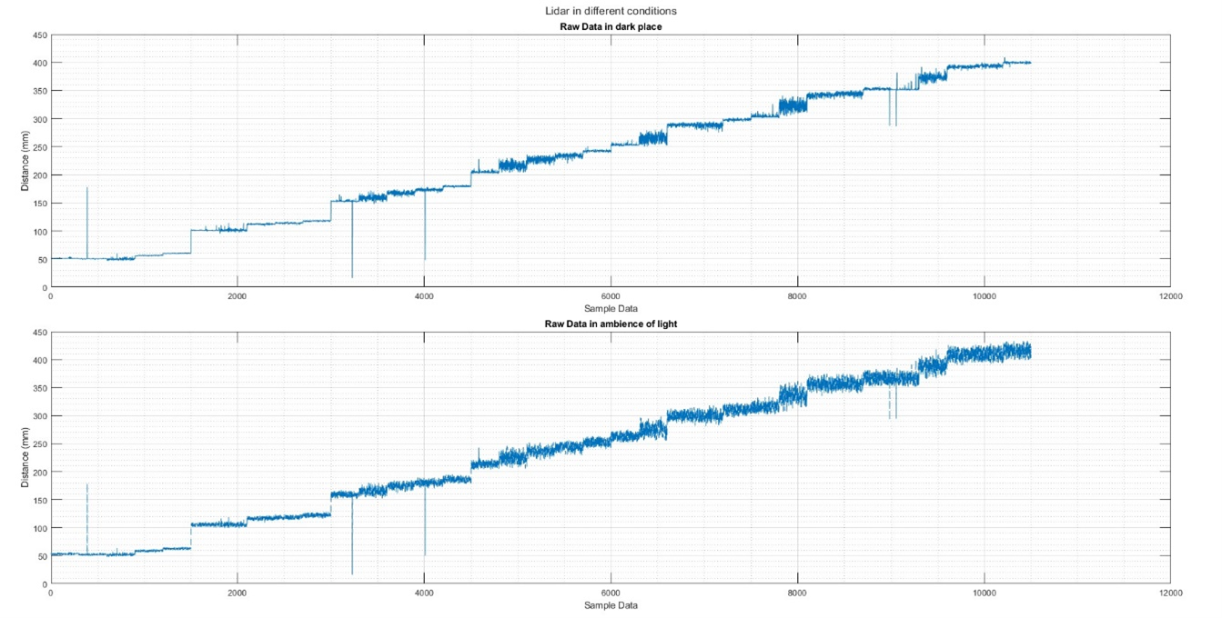
Figure 1. Raw Distance Measurement of LIDAR VL53L0X
Based on Table 1, this study selected the dark place parameter because it shows stable and meaningful variation with Standard deviation = 111.26 and Peak to peak range = 393. The Ambience of light parameter was excluded due to excessive noise across key metrics. It has higher raw fluctuation 6.78 from 2.65, more than double the high-frequency power 22.25 from 8.87, and larger adjacent differences 143.28 from 136. The noise is primarily introduced by ambient light variations that are unrelated to our measurement target. The dark place of raw LiDAR data had a measurement range from 16 to 409, with a mean value of 221.11 and a median value of 227. The difference between the minimum and maximum values produced a peak-to-peak range of 393, indicating that the data experienced considerable distance changes during the measurement process. This reason is well supported by previous research [41].
The standard deviation value of 111.26 also shows that the dispersion of the raw data was still wide. However, this value cannot be directly interpreted as pure noise because the data represent gradual changes in distance. Signal instability was more clearly indicated by the raw fluctuation value of 2.6457, the maximum adjacent difference of 136, and the detection of 81 spikes/drops in the raw data. In addition, the raw high-frequency power value of 8.8673 indicates the presence of rapid-change components in the signal. These findings support the visual observation in Figure 1 that the raw data still contained local fluctuations and sudden changes. Based on the visual observation and the initial characteristic parameters, the raw LiDAR data were not ideal for direct use as measurement output. Although the raw signal was still able to show the main pattern of distance change, the presence of local fluctuations, sudden value changes, and spikes/drops indicates that the signal still required improvement. Filtering was needed to suppress unstable variations, reduce rapid-change components, and clarify the main measurement pattern. Thus, the filtering stage became an important step before the LiDAR data were used for measurement performance analysis and sensor-based TVET learning applications.
Table 1. Raw LiDAR Data Characteristics
Parameter | Dark Place Value | Ambience of Light |
Minimum Value | 16 | 16.012 |
Maximum Value | 409 | 433.21 |
Mean raw value | 221.11 | 229.92 |
Standard deviation raw | 111.26 | 115.84 |
Peak-to-peak range | 393 | 417.2 |
Raw fluctuation | 2.6457 | 6.7771 |
Maximum adjacent difference | 136 | 143.28 |
Number of spike/drop | 81 | 81 |
High-frequency power raw | 8.8673 | 22.246 |
- Comparison of Raw and Filtered Distance Signals
At this stage, the raw LiDAR data were processed using five filtering methods, namely Moving Average, Median Filter, Savitzky-Golay, Butterworth, and Simple Kalman Filter. These five methods were applied to the same raw data so that changes in signal characteristics after the filtering process could be compared directly. This visual comparison is important because each filter has a different processing mechanism for reducing fluctuations, smoothing the signal, and preserving the main pattern of distance changes. Based on Figure 2, the raw signal still showed local fluctuations and relatively sharp value changes between samples. Although the main pattern of distance changes could still be identified, the raw signal was not sufficiently stable to be used directly as measurement output in sensor-based learning applications. This condition indicates that the filtering process is required to improve data readability and stability.
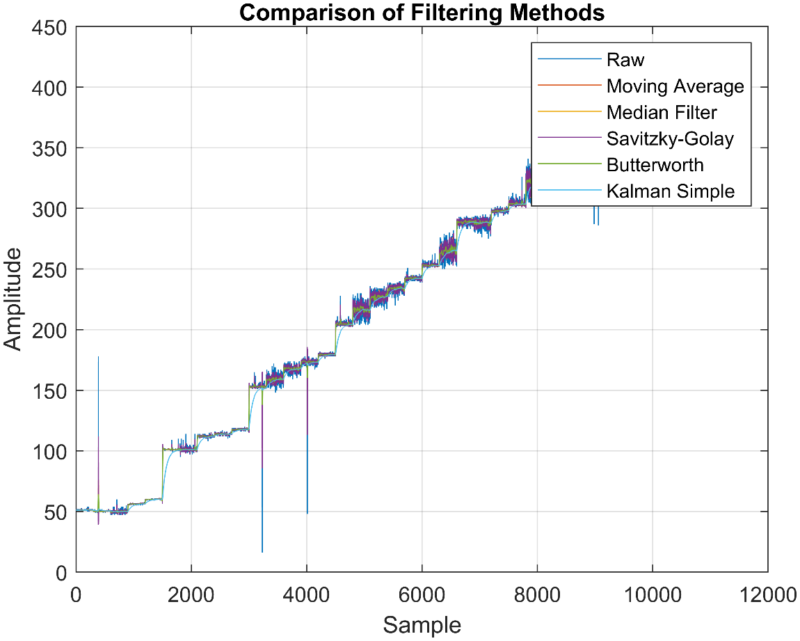
Figure 2. Raw and Filtered LiDAR Sensor Measurement Signals
The filtering results showed different characteristics for each method. Moving Average produced a smoother signal than the raw data while still following the main pattern of distance changes. The Median Filter was able to suppress local disturbances and temporary value spikes, although some signal variations were still visible. Savitzky-Golay provided a more balanced result because it could smooth the signal without removing the main shape of the measurement pattern. Meanwhile, Butterworth produced a very smooth signal by suppressing rapid-change or high-frequency components. However, its strong smoothing characteristic may reduce sensitivity to local changes. The Simple Kalman Filter produced the smoothest signal compared with the other methods, but a delayed response to distance changes was observed. This indicates that the Kalman Filter has strong smoothing capability, but it may reduce system responsiveness. In general, all filtering methods were able to improve the visual stability of the LiDAR signal. However, the degree of improvement differed across methods. Moving Average and Median Filter provided moderate smoothing, Savitzky-Golay maintained a balance between accuracy and signal shape, Butterworth was superior in suppressing high-frequency fluctuations, while the Simple Kalman Filter produced the smoothest signal but showed response delay.
- Residual Error and Signal Preservation Analysis
The first evaluation was conducted using error metrics, namely Mean Error Bias, Mean Absolute Error (MAE), Mean Squared Error (MSE), Root Mean Square Error (RMSE), Mean Absolute Percentage Error (MAPE), maximum absolute deviation, and steady-state error from the raw measurements. These metrics were used to determine the closeness of the filtered signals to the measurement reference value. The error evaluation results are presented in Table 2.
Table 2. Residual Error Relative for Each Filtering Method to Raw Data
Filter | Mean Error Bias | MAE | MSE | RMSE | MAPE (%) | Max absolute deviation | Steady-State Error |
Moving Average | 0,000017 | 1,7348 | 11,985 | 3,4620 | 0,9188 | 109,40 | 1,5372 |
Median Filter | -0,010143 | 1,5284 | 13,776 | 3,7116 | 0,8089 | 136,00 | 1,3877 |
Savitzky-Golay | -0,000011 | 1,3792 | 7,5316 | 2,7444 | 0,7219 | 69,686 | 1,2803 |
Butterworth | -0,000125 | 1,8485 | 13,299 | 3,6467 | 0,9921 | 122,01 | 1,6427 |
Kalman Simple | 2,1218 | 3,2774 | 35,103 | 5,9248 | 1,8236 | 133,96 | 2,8015 |
Based on Table 2, the Savitzky–Golay filter produced the smallest overall deviation from the raw LiDAR measurements. Its consistently low values across the absolute, squared, and percentage-based deviation metrics indicate that this method altered the original signal less than the other filters while still reducing fluctuations. The comparatively low maximum deviation also suggests that the Savitzky–Golay filter was better able to limit large pointwise changes between the raw and filtered signals. Therefore, this method provided the strongest balance between smoothing and preservation of the original measurement characteristics.
The Median Filter also showed relatively small deviations from the raw measurements. This behavior indicates that it was effective in removing local disturbances and isolated spikes without substantially modifying most of the signal. However, its larger maximum deviation shows that considerable changes still occurred at certain samples, particularly around abrupt transitions or transient events. This suggests that the Median Filter may preserve the general signal pattern while strongly modifying individual observations that it identifies as outliers.
The Moving Average and Butterworth filters showed moderate deviation performance. The Moving Average reduced local variations by averaging neighboring samples, but this process may also attenuate sharp transitions and introduce differences around rapidly changing regions. The Butterworth filter produced a smoother output, yet its higher deviation metrics indicate that stronger smoothing caused a greater departure from the original signal. This demonstrates that increased smoothness does not necessarily imply better preservation of the measured data.
The Simple Kalman Filter produced the greatest deviation from the raw measurements and also exhibited a noticeable directional offset. This suggests that the selected process-noise and measurement-noise parameters caused the filter to respond more slowly to changes in the input signal and to modify the signal level more substantially. Although the Kalman output was very smooth, the large deviation values indicate a greater loss of short-term variation and a weaker ability to follow rapid measurement changes under the parameter configuration used in this study.
After Table 2 shows numerical differences in residual error among the filtering methods, descriptive values alone are not sufficient to determine whether the observed differences are statistically significant. Therefore, an additional inferential analysis was conducted using a one way repeated measures analysis of variance. The raw LiDAR signal was divided into 42 non-overlapping segments of 250 samples, and the residual RMSE between each filtered output and the corresponding raw-signal segment was calculated. Because all filtering methods were applied to the same signal segments, the filtering method was treated as a within subject factor in the repeated measures ANOVA. Before interpreting the repeated-measures ANOVA, the sphericity assumption was examined using Mauchly’s test. The test result was significant, with Mauchly’s  , chi-square (9) = 404.38, and p < 0.001. This result indicates that the sphericity assumption was not satisfied. Therefore, the Greenhouse–Geisser correction was used, with an epsilon value of 0.274. As summarized in Table 3, the corrected repeated-measures ANOVA showed that the filtering method had a statistically significant effect on residual RMSE relative to the raw LiDAR signal,
  (1.10, 44.92) = 26.23, p < 0.001, with a partial eta-squared value of 0.390. These findings indicate that the differences in residual RMSE among the five filtering methods were statistically significant and were unlikely to be caused only by random variation among the signal segments.
Table 3. Repeated measures ANOVA results for segment level residual RMSE
Statistical analysis | Statistic | df | p-value | Additional information |
Mauchly’s test | 
| 9 | (<0.001) | Sphericity violated |
Greenhouse–Geisser correction | — | — | — | 
|
Repeated-measures ANOVA | ( ) ) | 1.10, 44.92 | (<0.001) | Partial  |
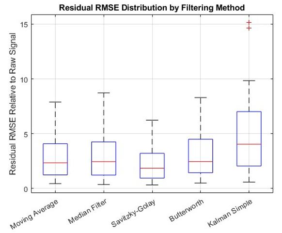
The descriptive results showed that the Savitzky–Golay filter produced the lowest mean residual RMSE, with a value of 2.249 ± 1.592. It was followed by Moving Average at 2.858 ± 1.977, Median Filter at 2.994 ± 2.220, Butterworth at 3.036 ± 2.044, and Simple Kalman Filter at 4.763 ± 3.566. As shown in Table 4, Savitzky–Golay also had the lowest median residual RMSE, whereas the Simple Kalman Filter showed the highest mean and median values. These results indicate that Savitzky–Golay preserved the raw-signal pattern more closely than the other filtering methods, while the Simple Kalman Filter produced the greatest deviation from the raw signal. The distribution of segment-level residual RMSE values is presented in Figure 3. As shown in Figure 3, Savitzky–Golay generally produced lower residual RMSE values and a narrower distribution than the other filtering methods. In contrast, the Simple Kalman Filter showed the highest median residual RMSE, the widest distribution, and several large values, indicating a greater degree of modification relative to the raw signal.
Table 4. Descriptive statistics of segment-level residual RMSE
Filtering method | Mean residual RMSE | Standard deviation | Median residual RMSE |
Moving Average | 2.858 | 1.977 | 2.328 |
Median Filter | 2.994 | 2.220 | 2.441 |
Savitzky–Golay | 2.249 | 1.592 | 1.840 |
Butterworth | 3.036 | 2.044 | 2.445 |
Simple Kalman Filter | 4.763 | 3.566 | 4.029 |
Figure 3. Distribution of segment-level residual RMSE relative to the raw signal across filtering methods
Bonferroni-adjusted post-hoc comparisons showed that the residual RMSE of Savitzky–Golay was significantly lower than that of Moving Average, Median Filter, Butterworth, and Simple Kalman Filter, with all adjusted p-values below 0.001. Table 5 also shows that the Simple Kalman Filter had a significantly higher residual RMSE than all other methods. No statistically significant difference was found between Moving Average and Median Filter, p = 0.102, or between Median Filter and Butterworth, p = 1.000.
Table 5. Bonferroni-adjusted post-hoc comparisons of residual RMSE
Pairwise comparison | Mean difference | Adjusted p-value | Result |
Moving Average vs Median Filter | −0.136 | 0.102 | Not significant |
Moving Average vs Savitzky–Golay | 0.609 | (<0.001) | Significant |
Moving Average vs Butterworth | −0.178 | (<0.001) | Significant |
Moving Average vs Simple Kalman | −1.905 | (<0.001) | Significant |
Median Filter vs Savitzky–Golay | 0.745 | (<0.001) | Significant |
Median Filter vs Butterworth | −0.042 | 1.000 | Not significant |
Median Filter vs Simple Kalman | −1.769 | (<0.001) | Significant |
Savitzky–Golay vs Butterworth | −0.788 | (<0.001) | Significant |
Savitzky–Golay vs Simple Kalman | −2.514 | (<0.001) | Significant |
Butterworth vs Simple Kalman | −1.727 | (<0.001) | Significant |
Therefore, the post-hoc results confirm that Savitzky–Golay provided the highest level of raw-signal preservation among the evaluated filtering methods. It should be noted that the residual RMSE used in this analysis does not represent measurement accuracy relative to the actual distance because an independent ground-truth reference was not available. Instead, the metric indicates the degree of deviation between each filtered output and the raw LiDAR signal. A lower residual RMSE therefore reflects stronger preservation of the original signal pattern, while a higher value indicates that the filtering method modified the raw signal more extensively. Consequently, the results of this analysis should be interpreted together with the signal-stability, noise-reduction, and responsiveness indicators presented in the following sections. This combined interpretation is necessary because a filter that remains very close to the raw signal may also retain unwanted fluctuations, whereas a filter that produces a smoother signal may introduce greater deviation or response delay.
- Signal Stability and Smoothness Analysis
Signal stability was evaluated using standard deviation, standard deviation reduction, signal fluctuation, fluctuation reduction, and smoothness index. These metrics are important because sensor-based learning applications require data that are stable, easy to read, and not excessively fluctuating. The results of the signal stability evaluation are presented in Table 6.
Table 6. Evaluation of Deviation to Raw Measurements
Filter | STD Raw | STD Filter | STD Reduction (%) | Fluctuation Raw | Fluctuation Filter | Fluctuation Reduction (%) | Smoothness Index |
Moving Average | 111,26 | 111,20 | 0,0539 | 5,4607 | 1,1441 | 79,048 | 1,1446 |
Median Filter | 111,26 | 111,23 | 0,0270 | 5,4607 | 1,4686 | 73,106 | 1,4689 |
Savitzky-Golay | 111,26 | 111,22 | 0,0360 | 5,4607 | 2,5654 | 53,021 | 2,5655 |
Butterworth | 111,26 | 111,19 | 0,0629 | 5,4607 | 0,3029 | 94,453 | 0,3047 |
Kalman Simple | 111,26 | 111,00 | 0,2337 | 5,4607 | 0,0865 | 98,416 | 0,0927 |
Based on Table 6, the global standard deviation values of all filtered signals did not show substantial changes compared with the raw data. This occurred because the measurement data had a considerable distance-change trend during the data collection process. Therefore, the global standard deviation does not fully represent noise, but also reflects the distance changes that actually occurred during measurement. More relevant indicators for evaluating local stability are fluctuation values and the smoothness index. Based on these indicators, the Simple Kalman Filter produced the smoothest result, with a fluctuation reduction of 98.416% and a smoothness index of 0.0927. These values indicate that the Kalman Filter was highly effective in suppressing small changes between samples. Butterworth also showed very good performance in improving signal smoothness. This method produced a fluctuation reduction of 94.453% and a smoothness index of 0.3047. These results indicate that Butterworth was effective in suppressing local fluctuations and producing a stable output. Moving Average reduced fluctuation by 79.048%, while the Median Filter reduced fluctuation by 73.106%. Both methods provided a fairly good improvement in stability without excessively removing the main signal pattern. Meanwhile, Savitzky-Golay had the lowest fluctuation reduction, at 53.021%, with a smoothness index of 2.5655. However, this value does not directly indicate poor performance. Savitzky-Golay does not perform aggressive smoothing because this method attempts to preserve the local shape of the signal. Thus, if the main focus is signal smoothness as shown in Figure 4, the Simple Kalman Filter and Butterworth are the most superior methods. However, if stability needs to be balanced with accuracy and preservation of the signal shape, Savitzky-Golay remains an important method to consider.
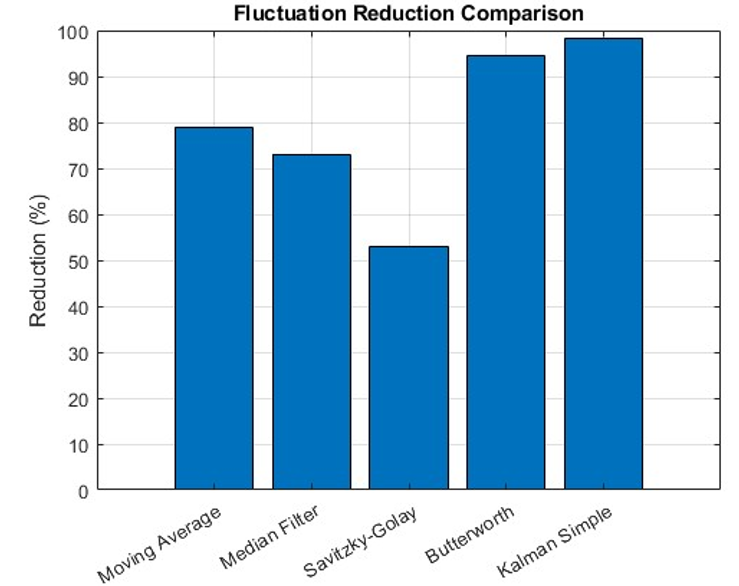
Figure 4. Comparison of Fluctuation Reduction Across Filtering Methods
- Residual Noise and High-Frequency Power Reduction Analysis
Noise reduction was evaluated using the standard deviation of residual noise, RMS residual noise, estimated Signal-to-Noise Ratio (SNR), and high-frequency power reduction. These metrics were used to determine the ability of each filter to reduce disturbance components contained in the LiDAR signal. The evaluation results are presented in Table 7.
Table 7. Evaluation of Residual Noise and High-Frequency Power Reduction
Filter | STD Residual Noise | RMS Residual Noise | Estimated SNR (dB) | HF Power Raw | HF Power Filter | HF Power Reduction (%) |
Moving Average | 3,4621 | 3,4620 | 30,135 | 0,0011669 | 0,00019937 | 82,914 |
Median Filter | 3,7118 | 3,7116 | 29,532 | 0,0011669 | 0,00023462 | 79,893 |
Savitzky-Golay | 2,7445 | 2,7444 | 32,154 | 0,0011669 | 0,00045215 | 61,250 |
Butterworth | 3,6469 | 3,6467 | 29,683 | 0,0011669 | 0,00017267 | 85,202 |
Kalman Simple | 5,5321 | 5,9248 | 26,048 | 0,0011669 | 0,00017231 | 85,233 |
Based on Table 7, Savitzky-Golay produced the lowest residual noise, with a residual noise STD of 2.7445 and an RMS residual noise of 2.7444. This method also produced the highest estimated SNR of 32.154 dB. These results indicate that Savitzky-Golay was able to reduce noise while maintaining signal conformity with the main measurement pattern. Butterworth and the Simple Kalman Filter showed the best performance in suppressing high-frequency power. Butterworth produced a high-frequency power reduction of 85.202%, while the Simple Kalman Filter produced a reduction of 85.233%. Both methods were effective in suppressing rapid-change components that are generally associated with noise or local fluctuations. However, a large reduction in high-frequency components does not always indicate better overall performance. Although the Simple Kalman Filter was able to suppress high-frequency power, it produced the highest RMS residual noise of 5.9248 and the lowest SNR of 26.048 dB. This indicates that the Kalman Filter smoothed the signal too strongly, which could reduce signal conformity with the reference pattern. Moving Average also showed fairly good performance, with a high-frequency power reduction of 82.914% and an estimated SNR of 30.135 dB. The Median Filter produced a high-frequency power reduction of 79.893% and an SNR of 29.532 dB. These values indicate that both methods were able to reduce noise, although they were not as effective as Savitzky-Golay in terms of residual noise and SNR. Overall, these results show that filter selection cannot be based solely on the ability to suppress high-frequency components. An overly aggressive filter may produce a very smooth signal but can also increase residual error. Based on the balance between residual noise and SNR, Savitzky-Golay provided the best performance in this study. As shown in Figure 5, the Butterworth and Simple Kalman filters achieved the highest high-frequency power reduction, whereas Savitzky–Golay produced the lowest reduction among the evaluated methods.
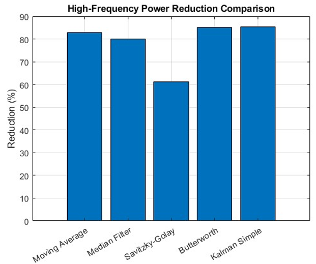
Figure 5. Comparison of High-Frequency Power Reduction
- Responsiveness and Transient Error Evaluation
Filter responsiveness was evaluated using lag samples and maximum transient error. This evaluation is important because sensor-based measurement systems in TVET learning require a fast response when distance changes occur. A filter that responds too slowly may reduce the quality of real-time feedback for students. The responsiveness evaluation results are presented in Table 8.
Table 8. Responsiveness and Transient Error Evaluation
Filter | Lag Samples | Max Deviation Transient |
Moving Average | 0 | 109,40 |
Median Filter | 0 | 136,00 |
Savitzky-Golay | 0 | 69,686 |
Butterworth | 0 | 122,01 |
Kalman Simple | 39 | 133,96 |
Based on Table 8, Moving Average, Median Filter, Savitzky-Golay, and Butterworth did not show response delay, with lag sample values of 0. This indicates that the four methods were able to follow the main pattern of signal changes without any delay detected based on the evaluation procedure used. Among these four methods, Savitzky-Golay produced the lowest maximum transient error, namely 69.686. This result indicates that Savitzky-Golay was more stable in following distance changes under transient conditions. In other words, this method was not only accurate under general conditions but was also able to maintain low error when changes in measurement values occurred. In contrast, the Simple Kalman Filter had a lag of 39 samples. With a sampling frequency of 50 Hz, this lag is equivalent to approximately 0.78 seconds. This delay is important in the context of sensor-based learning because students need data visualization that is responsive to changes in the observed object. Although the Simple Kalman Filter produced the smoothest signal, the presence of lag and high maximum transient error indicates a trade-off between smoothness and responsiveness. Therefore, the Kalman Filter configuration used in this study was not the best option for TVET learning applications that require fast response and good measurement accuracy.
- Overall Comparison and Selection Filter
The evaluation results show that each filtering method had its own strengths and weaknesses. Savitzky-Golay showed the best performance in terms of error metrics, residual noise, SNR, and transient response. This method produced the lowest MAE, MSE, RMSE, MAPE, Maximum Absolute Deviation, residual noise, and maximum transient error compared with the other methods. In addition, Savitzky-Golay did not show any lag in the evaluation results. Butterworth and the Simple Kalman Filter were superior in terms of signal smoothing. Butterworth was able to reduce fluctuation by 94.454% and high-frequency power by 85.202%. The Simple Kalman Filter even produced the highest fluctuation reduction of 98.415% and high-frequency power reduction of 85.233%. However, these advantages were accompanied by limitations. The Kalman Filter produced higher error, lower SNR, and a lag of 39 samples. Thus, the Kalman Filter was not the best method when accuracy and responsiveness were considered simultaneously. Moving Average provided fairly stable and simple performance. This method is suitable when the system requires a filter that is easy to implement and easy to understand in the context of basic learning. The Median Filter was fairly effective in reducing local disturbances or outliers, but its high Maximum Absolute Deviation and transient error values indicate that this method was less stable under certain signal changes. Based on the comprehensive evaluation, Savitzky-Golay is recommended as the best filtering method in this study. This method provides the best balance among accuracy, stability, noise reduction, and responsiveness. Butterworth can be used when the main priority is to produce a very smooth signal, while Moving Average can be used when the priority is implementation simplicity. The Simple Kalman Filter still requires further parameter tuning to be used optimally in real-time signal processing systems.
- Implications of the Results for TVET Learning Applications
Based on the evaluation results, the implementation of each filtering method should be adjusted according to the specific requirements of the system. The findings indicate that each filter has distinct strengths and limitations; therefore, filter selection cannot be based on a single performance indicator alone. In sensor-based TVET learning applications, measurement data must not only be smooth but also accurate, responsive, and easy for students to interpret. Consequently, the choice of filtering method should consider the primary objective of the system, whether it emphasizes measurement accuracy, visual stability, noise reduction, responsiveness to changes, or ease of implementation.
Moving Average is more suitable for systems that require a simple, low computational cost, and easily implemented filtering method [42][43]. The evaluation results showed that Moving Average reduced fluctuations by 79.047% and reduced high-frequency power by 82.914% without introducing lag. These findings indicate that Moving Average can be used when sensor data contain mild to moderate random fluctuations and the system requires a more stable signal display with low computational complexity. In the context of TVET learning, this filter is suitable for introducing the basic concept of data smoothing because its mechanism is easy for students to understand. However, Moving Average is not the preferred option when the highest measurement accuracy is required, since its MAE and RMSE values are still higher than those of Savitzky-Golay.
The Median Filter is more appropriate when sensor data contain extreme spikes, sudden drops, or outliers. This is consistent with the characteristic of the Median Filter, which selects the median value within a data window, making the output less affected by extreme values [44][45]. Based on the evaluation results, the Median Filter produced an MAE of 1.5284 and a MAPE of 0.8089%, which are better than those of Moving Average and Butterworth in terms of absolute error. Therefore, the Median Filter may be selected when the main disturbances in LiDAR data are temporary outliers caused by surface reflections, changes in measurement angle, or unstable sensor readings at specific points. However, the Median Filter is less suitable when a very smooth signal is required because its fluctuation reduction was only 73.105%. In addition, its maximum transient error of 136 indicates that the filter may still produce large deviations under certain signal-change conditions.
Savitzky-Golay is more suitable when the system requires a balance between accuracy, signal shape preservation, and responsiveness [46][47]. The evaluation results showed that Savitzky-Golay produced the lowest MAE of 1.3792, the lowest RMSE of 2.7444, the lowest MAPE of 0.7219%, the lowest Maximum Absolute Deviation of 69.686, and the highest estimated SNR of 32.154 dB. This filter also showed no lag and had the lowest maximum transient error among all evaluated methods. These results indicate that Savitzky-Golay is well suited for LiDAR measurements involving gradual changes, such as water-level variations, because it can reduce noise without removing the main trend of the signal. In TVET learning applications, this method is particularly appropriate when students need to observe the relationship between changes in physical objects and sensor outputs with a high degree of accuracy. However, Savitzky-Golay is not the primary choice when the main priority is achieving the smoothest possible visual signal, since its fluctuation reduction was only 53.021%, lower than that of Butterworth and the Simple Kalman Filter.
Butterworth filtering is particularly suitable when the primary objective is to attenuate high-frequency noise and produce a smoother signal while preserving its essential low-frequency characteristics [48][49]. The evaluation results showed that Butterworth reduced fluctuations by 94.454% and high-frequency power by 85.202%. These achievements indicate that Butterworth is effective for sensor data containing substantial rapid fluctuations or high-frequency noise. This filter is suitable for learning applications that emphasize signal display stability so that graphical outputs are easier to interpret. However, Butterworth produced an MAE of 1.8485 and an RMSE of 3.6467, indicating lower accuracy than Savitzky-Golay. Therefore, Butterworth is more suitable when signal smoothness and high-frequency noise reduction are the primary objectives rather than minimizing measurement error.
The Simple Kalman Filter is particularly suitable for systems that prioritize smooth and stable state estimation from noisy sequential measurements [50]. The evaluation results showed that the Simple Kalman Filter achieved the highest fluctuation reduction of 98.415% and the lowest smoothness index of 0.09268. These results indicate that the filter is highly effective in producing a smooth output signal. However, these advantages are accompanied by limitations in accuracy and responsiveness. The Simple Kalman Filter produced an MAE of 3.2774, an RMSE of 5.9248, a MAPE of 1.8236%, and a lag of 39 samples. With a sampling frequency of 50 Hz, this lag corresponds to approximately 0.78 seconds. These findings indicate that the Kalman Filter configuration used in this study is less suitable for systems requiring rapid responses to distance changes. Therefore, the Simple Kalman Filter is more appropriate for relatively slow and stable measurement conditions or when visual smoothness is more important than real-time responsiveness.
Recent sensor-processing studies have increasingly investigated adaptive filters that adjust their parameters according to changes in signal and noise characteristics. Unlike the fixed-parameter Simple Kalman Filter used in this study, an adaptive Kalman Filter can estimate or update process and measurement noise covariance during operation. Kruse et al. proposed an adaptive Kalman filtering approach that estimates process and measurement noise covariance using Kalman smoothing. This adaptive capability is relevant to VL53L0X measurements because LiDAR noise may vary with object reflectivity, measurement angle, ambient light, distance, and surface movement. The fixed Q and R values applied in the present Simple Kalman Filter produced strong fluctuation reduction but also generated higher error and a lag of 39 samples [51]. AI-based and hybrid filtering techniques offer another alternative. Zhang et al. integrated a Long Short-Term Memory network with an adaptive Kalman Filter to estimate dynamic states under nonlinear and changing operating conditions. In this approach, the learning model supports the filter in adjusting its estimation process according to temporal signal patterns [52]. Such hybrid methods may be useful when sensor disturbances cannot be adequately represented by fixed statistical assumptions. Future research should therefore compare the present conventional filters with adaptive Kalman filtering, adaptive window-based filters, neural denoising models, and hybrid neural-Kalman approaches using the same VL53L0X dataset and identical evaluation indicators.
Overall, the results of this study demonstrate that the selection of a filtering method should be based on implementation requirements. Moving Average is suitable for simple and lightweight systems, the Median Filter is suitable for data containing outliers or spikes, Savitzky-Golay is suitable for measurements requiring accuracy and signal pattern preservation, Butterworth is suitable for high-frequency noise reduction, and the Simple Kalman Filter is suitable for highly smooth signal estimation but requires further parameter tuning to avoid response delays. Therefore, the implementation of filters in sensor-based TVET learning applications should not treat a single method as a universal solution, but rather as a technical option selected according to data characteristics, learning objectives, and system responsiveness requirements.
- CONCLUSION
This study evaluated the performance of five filtering methods, namely Moving Average, Median Filter, Savitzky-Golay, Butterworth, and Simple Kalman Filter, in improving the quality of measurement data obtained from a VL53L0X LiDAR sensor for sensor-based TVET learning applications. The initial characterization showed that the raw LiDAR signal contained local fluctuations, abrupt sample-to-sample changes, and high-frequency components that reduced the stability and readability of the measurements. Each filtering method was therefore applied to the same raw dataset, and its performance was evaluated by comparing the filtered output with the corresponding raw signal. The comparison focused on the extent to which each method reduced fluctuations and high-frequency components while preserving the main characteristics of the original measurements.
The results showed that Savitzky–Golay provided the most balanced performance. It produced an MAE of 1.3792, an RMSE of 2.7444, a MAPE of 0.7219%, a maximum absolute deviation of 69.686, the highest estimated SNR of 32.154 dB, and no detected lag. A Greenhouse–Geisser-corrected repeated-measures ANOVA confirmed that the filtering method had a statistically significant effect on segment-level residual RMSE, F(1.10,44.92)=26.23, p<0.001, partial η2=0.390. Bonferroni-adjusted comparisons further showed that Savitzky–Golay produced significantly lower residual RMSE than the other methods, indicating the strongest preservation of the raw-signal pattern.
Butterworth and the Simple Kalman Filter demonstrated advantages in signal smoothing. Butterworth reduced fluctuations by 94.454% and high-frequency power by 85.202%, while the Simple Kalman Filter achieved the highest fluctuation reduction of 98.415% and the lowest smoothness index of 0.09268. However, the Simple Kalman Filter also produced an MAE of 3.2774, an RMSE of 5.9248, a MAPE of 1.8236%, and a lag of 39 samples. These findings indicate that the smoothest filter is not necessarily the most appropriate choice for systems requiring fast response and low deviation from the reference signal.
Moving Average and Median Filter offered advantages in terms of implementation simplicity. Moving Average reduced fluctuations by 79.047% and high-frequency power by 82.914%, making it suitable for systems requiring low computational complexity and basic signal smoothing. The Median Filter was more suitable when the data contained temporary spikes, drops, or outliers because it uses the median value within the observation window. However, the Median Filter still produced relatively high Maximum Absolute Deviation and transient error values, indicating that its application should be carefully considered in systems operating under rapid distance-change conditions.
Overall, no single filtering method was superior across all indicators. Savitzky–Golay is recommended when signal-pattern preservation and responsiveness are the main priorities, Butterworth when stronger high-frequency suppression is required, Simple Kalman when maximum smoothness is preferred and delay is acceptable, Moving Average for simple instructional implementation, and Median Filter for impulsive disturbances. Because the raw signal was used as the comparison signal rather than an independent ground-truth measurement, the reported residual metrics represent signal preservation and deviation from the raw data, not measurement accuracy relative to the actual distance.
Future research should evaluate the filtering methods under different environmental conditions, including variations in ambient light, object reflectivity, measurement angle, surface characteristics, and sensor-to-object distance. Experiments involving static and dynamic objects are also required to assess filter performance under faster and more complex distance changes. Further studies should compare additional LiDAR sensor models to determine whether the findings can be generalized across devices with different measurement ranges, resolutions, and acquisition mechanisms. Adaptive filtering techniques may also be investigated to enable automatic parameter adjustment according to changing noise and signal characteristics. Finally, real-time implementation on embedded platforms should be examined through computational benchmarking that includes processing time, memory usage, processor load, energy consumption, sampling consistency, and end-to-end latency. These developments would support the implementation of more reliable, responsive, and scalable LiDAR-based learning systems in TVET environments.
ACKNOWLEDGEMENT
The authors would like to express their gratitude to all parties who assisted in the data collection process, the testing of the LiDAR sensor system, and the analysis of the filtering results, enabling this study to be completed successfully.
REFERENCES
- J. Cai and M. Kosaka, “Conceptualizing Technical and Vocational Education and Training as a Service Through Service-Dominant Logic,” Sage Open, vol. 14, no. 2, 2024, https://doi.org/10.1177/21582440241240847.
- S. Park and H. Park, “Capacity Building of TVET Trainers in a Developing Country Through Practice-oriented Curriculum Implementation,” Journal of Technical Education and Training, vol. 17, no. 4, pp. 135–147, 2025, https://doi.org/10.30880/jtet.2025.17.04.011.
- R. Parua and W. Yang, “The Driving Logic of Digital Transformation in TVET,” Vocation, Technology & Education, vol. 1, no. 2, p. e17, 2024, https://doi.org/10.54844/vte.2024.0590.
- M. J. Gomez, J. A. Ruipérez-Valiente, and F. J. García Clemente, “Exploring Technology- and Sensor-Driven Trends in Education: A Natural-Language-Processing-Enhanced Bibliometrics Study,” Sensors, vol. 23, no. 23, p. 9303, 2023, https://doi.org/10.3390/s23239303.
- P. A. García-Tudela and J.-A. Marín-Marín, “Use of Arduino in Primary Education: A Systematic Review,” Educ. Sci. (Basel)., vol. 13, no. 2, p. 134, 2023, https://doi.org/10.3390/educsci13020134.
- D. Hercog, T. Lerher, M. Truntič, and O. Težak, “Design and Implementation of ESP32-Based IoT Devices,” Sensors, vol. 23, no. 15, p. 6739, 2023, https://doi.org/10.3390/s23156739.
- M. Bleier, “Sensor Cube: A Tool for Hands-on Learning of Sensor Data Processing,” IFAC-PapersOnLine, vol. 58, no. 16, pp. 23–28, 2024, https://doi.org/10.1016/j.ifacol.2024.08.456.
- T. Panskyi, E. Korzeniewska, and A. Firych-Nowacka, “Educational Data Clustering in Secondary School Sensor-Based Engineering Courses Using Active Learning Approaches,” Applied Sciences, vol. 14, no. 12, p. 5071, 2024, https://doi.org/10.3390/app14125071.
- L. G. Trujillo-Franco, H. F. Abundis-Fong, and J. C. Marin-Soriano, “An Open-Source Data Acquisition Platform for Teaching Vibration Analysis,” Computer Applications in Engineering Education, vol. 32, no. 5, p. e22753, 2024, https://doi.org/10.1002/cae.22753.
- M. J. Silva, C. Gouveia, and C. A. Gomes, “The Use of Mobile Sensors by Children: A Review of Two Decades of Environmental Education Projects,” Sensors, vol. 23, no. 18, p. 7677, 2023, https://doi.org/10.3390/s23187677.
- M. A. Hernández-Mustieles et al., “Wearable Biosensor Technology in Education: A Systematic Review,” Sensors, vol. 24, no. 8, p. 2437, 2024, https://doi.org/10.3390/s24082437.
- X. Zhang, Y. Ding, X. Huang, W. Li, L. Long, and S. Ding, “Smart Classrooms: How Sensors and AI Are Shaping Educational Paradigms,” Sensors, vol. 24, no. 17, p. 5487, 2024, https://doi.org/10.3390/s24175487.
- P. Sun, C. Sun, R. Wang, and X. Zhao, “Object Detection Based on Roadside LiDAR for Cooperative Driving Automation: A Review,” Sensors, vol. 22, no. 23, p. 9316, 2022, https://doi.org/10.3390/s22239316.
- N. Lopac, I. Jurdana, A. Brnelić, and T. Krljan, “Application of Laser Systems for Detection and Ranging in the Modern Road Transportation and Maritime Sector,” Sensors, vol. 22, no. 16, p. 5946, 2022, https://doi.org/10.3390/s22165946.
- D. Wisth, M. Camurri, and M. Fallon, “VILENS: Visual, Inertial, Lidar, and Leg Odometry for All-Terrain Legged Robots,” IEEE Transactions on Robotics, vol. 39, pp. 309–326, Jul. 2022, https://doi.org/10.1109/TRO.2022.3193788.
- S. Jiang et al., “Navigation system for orchard spraying robot based on 3D LiDAR SLAM with NDT_ICP point cloud registration,” Comput. Electron. Agric., vol. 220, p. 108870, 2024, https://doi.org/10.1016/j.compag.2024.108870.
- J. A. Ruipérez-Valiente, R. Martínez-Maldonado, D. Di Mitri, and J. Schneider, “From Sensor Data to Educational Insights,” Sensors, vol. 22, no. 21, p. 8556, 2022, https://doi.org/10.3390/s22218556.
- M. Lötscher, N. Baumann, E. Ghignone, A. Ronco, and M. Magno, “Assessing the Robustness of LiDAR, Radar and Depth Cameras Against Ill-Reflecting Surfaces in Autonomous Vehicles: An Experimental Study,” in 2023 IEEE International Conference on Omni-layer Intelligent Systems, 2023. https://doi.org/10.1109/COINS57856.2023.10189236.
- T. T. Nguyen, V. T. Nguyen, and H. Kim, “Improvement of Accuracy and Precision of the LiDAR System Working in High Background Light Conditions,” Electronics (Basel)., vol. 11, no. 1, p. 45, 2021, https://doi.org/10.3390/electronics11010045.
- V. G. Biju and others, “Assessing the Influence of Sensor-Induced Noise on Machine Learning Accuracy,” Sensors, vol. 24, no. 2, p. 330, 2024, https://doi.org/10.3390/s24020330.
- L. Türkler and L. Ö. Akkan, “Noise Reduction Techniques for Sensor Data: Comparative Analysis of Kalman, Butterworth, Savitzky-Golay, Median, and Moving Average Filters for UWB-Based Position Estimation,” Celal Bayar University Journal of Science, vol. 21, no. 4, pp. 146–159, 2025, https://doi.org/10.18466/cbayarfbe.1682594.
- M. H. Raju, “Filtering Eye-Tracking Data From an EyeLink 1000,” Vision, vol. 14, no. 3, p. 17, 2023, https://doi.org/10.3390/vision14030017.
- A. E. Hurtado-Perez and others, “Use of Technologies for the Acquisition and Processing of Sensor Data: A Review,” Biomimetics, vol. 10, no. 5, p. 339, 2025, https://doi.org/10.3390/biomimetics10050339.
- A. J. Kałka and A. M. Turek, “Searching for Alternatives to the Savitzky–Golay Filter in the Spectral Processing Domain,” Appl. Spectrosc., vol. 77, no. 4, pp. 426–432, 2023, https://doi.org/10.1177/00037028231154278.
- M. H. Raju, L. Friedman, T. M. Bouman, and O. V Komogortsev, “Filtering Eye-Tracking Data from an EyeLink 1000: Comparing Heuristic, Savitzky–Golay, IIR, and FIR Digital Filters,” J. Eye Mov. Res., vol. 14, no. 3, p. 6, 2023, https://doi.org/10.16910/jemr.14.3.6.
- G. Takács, E. Mikuláš, M. Gulan, A. Vargová, and J. Boldocký, “AutomationShield: An Open-Source Hardware and Software Initiative for Control Engineering Education,” IFAC-PapersOnLine, vol. 56, no. 2, pp. 9594–9599, 2023, https://doi.org/10.1016/j.ifacol.2023.10.263.
- F. Baskoro, I. G. P. A. Buditjahjanto, M. Rohman, D. A. S. Fridyatama, and A. P. Nurdiansyah, “Impact of Sample Size Variation on Moving Average Filter Performance for Stability and Accuracy in Ultrasonic Sensor Measurements,” TEM Journal, vol. 14, no. 2, pp. 1681–1688, 2025, https://doi.org/10.18421/TEM142-65.
- F. Baskoro, M. Rohman, D. Arya, and A. Putra, “Optimizing Stability of Ultrasonic Sensor Readings: Study on Moving Average Filter Parameter Selection,” JOURNAL ZETROEM, vol. 7, no. 1, pp. 59–65, Mar. 2025, https://doi.org/10.36526/ztr.v7i1.3603.
- N. Ariyanto, F. Baskoro, R. Firmansyah, L. Anifah, T. Wrahatnolo, and D. A. S. Fridyatama, “Trade-Off Analysis of Moving Average Filter in Light Sensors,” Engineering Science Letter, vol. 5, no. 02, pp. 103–109, Jun. 2026, https://doi.org/10.56741/IISTR.esl.002255.
- N. Li and others, “An Improved Adaptive Median Filtering Algorithm for Radar Co-Channel Interference,” Sensors, vol. 22, no. 19, p. 7573, 2022, https://doi.org/10.3390/s22197573.
- N. Hublikar and A. Gupta, “Comparative Analysis of Median, Gaussian, and Butterworth Filters Under Consistent and Varying Noise Conditions at Multiple Filter Sizes,” Jul. 2025, pp. 1–4. https://doi.org/10.1109/ICITEICS64870.2025.11341237.
- M. M. Elgaud et al., “Digital Filtering Techniques for Performance Improvement of Golay Coded TDM-FBG Sensor,” Sensors, vol. 21, no. 13, p. 4299, 2021, https://doi.org/10.3390/s21134299.
- Y. Rawash, B. Al-Naami, A. Alfraihat, and H. Owida, “Advanced Low-Pass Filters for Signal Processing: A Comparative Study on Gaussian, Mittag-Leffler, and Savitzky-Golay Filters,” Mathematical Modelling of Engineering Problems, vol. 11, pp. 1841–1850, Jul. 2024, https://doi.org/10.18280/mmep.110713.
- L. Zhao, H. Yuan, K. Xu, J. Bi, and B. H. Li, “Hybrid network attack prediction with Savitzky–Golay filter-assisted informer,” Expert Syst. Appl., vol. 235, p. 121126, 2024, https://doi.org/10.1016/j.eswa.2023.121126.
- C.-S. Huang and others, “An Adaptive Cutoff Frequency Design for Butterworth Low-Pass Filter Pursuing Robust Parameter Identification for Battery Energy Storage Systems,” Batteries, vol. 9, no. 4, p. 198, 2023, https://doi.org/10.3390/batteries9040198.
- D. Suescún-Díaz, G. Ule-Duque, and L. E. Cardoso-Páez, “Butterworth Filter to Reduce Reactivity Fluctuations,” Karbala International Journal of Modern Science, vol. 10, no. 1, pp. 91–98, 2024, https://doi.org/10.33640/2405-609X.3342.
- O. J. Montañez and others, “Application of Data Sensor Fusion Using Extended Kalman Filter Algorithm for Identification and Tracking of Moving Targets from LiDAR–Radar Data,” Remote Sens. (Basel)., vol. 15, no. 13, p. 3396, 2023, https://doi.org/10.3390/rs15133396.
- A. Chhabra and others, “Measurement Noise Covariance-Adapting Kalman Filters for Varying Sensor Noise Situations,” Sensors, vol. 21, no. 24, p. 8304, 2021, https://doi.org/10.3390/s21248304.
- D. Voipan, A. E. Voipan, and M. Barbu, “Evaluating Machine Learning-Based Soft Sensors for Effluent Quality Prediction in Wastewater Treatment Under Variable Weather Conditions,” Sensors, vol. 25, no. 6, p. 1692, 2025, https://doi.org/10.3390/s25061692.
- A. Tungatarova, G. Borankulova, A. Murzakhmetov, and B. Turarova, “Hybrid IoT-VIoT System for Real-Time Water-Level Monitoring Using Computer Vision,” Computers, vol. 15, no. 6, p. 373, 2026, https://doi.org/10.3390/computers15060373.
- S. Komarizadehasl, B. Mobaraki, H. Ma, J.-A. Lozano-Galant, and J. Turmo, “Low-Cost Sensors Accuracy Study and Enhancement Strategy,” Applied Sciences, vol. 12, no. 6, 2022, https://doi.org/10.3390/app12063186.
- L. Xiong, T. Zhang, A. Yuan, and Z. Zhang, “Research on Filtering Algorithm of Vehicle Dynamic Weighing Signal,” World Electric Vehicle Journal, vol. 15, no. 6, p. 254, 2024, https://doi.org/10.3390/wevj15060254.
- L. Huang, D. Li, H. Yan, K. Wang, and Z. Huang, “A Low-Complexity Forward–Backward Filtering Algorithm for Real-Time GNSS Deformation Monitoring at the Edge,” Electronics (Basel)., vol. 14, no. 12, p. 2388, 2025, https://doi.org/10.3390/electronics14122388.
- M. Jung and D.-Y. Kim, “DEFT: A Dynamic Environmental Filtering and Thresholding Algorithm for Adaptive Headlamp Control Using Ride Height Sensors,” Electronics (Basel)., vol. 13, no. 23, p. 4788, 2024, https://doi.org/10.3390/electronics13234788.
- S. Kumar, R. Raja, M. R. Mahmood, and S. Choudhary, “A Hybrid Method for the Removal of RVIN Using Self Organizing Migration with Adaptive Dual Threshold Median Filter,” Sens. Imaging, vol. 24, no. 1, p. 9, 2023, https://doi.org/10.1007/s11220-023-00414-9.
- A. Kenioua, O. Djebili, and A. T. Brahim, “Hybrid Extreme Learning Machine for Real-Time Rate of Penetration Prediction,” J. Pet. Explor. Prod. Technol., vol. 15, p. 139, 2025, https://doi.org/10.1007/s13202-025-02048-x.
- N. Ádám, D. Val’ko, Z. Balogh, B. Madoš, and J. Hurtuk, “Comparative Evaluation of Filtration Techniques for ECG Signal Denoising with Emphasis on Stationary Wavelet Transform,” Sci. Rep., vol. 15, p. 42514, 2025, https://doi.org/10.1038/s41598-025-26476-1.
- D. Khan et al., “Robust Human Locomotion and Localization Activity Recognition over Multisensory,” Front. Physiol., vol. 15, p. 1344887, 2024, https://doi.org/10.3389/fphys.2024.1344887.
- S. Ellens, D. L. Carey, P. B. Gastin, and M. C. Varley, “Accuracy of GNSS-Derived Acceleration Data for Dynamic Team Sport Movements: A Comparative Study of Smoothing Techniques,” Applied Sciences, vol. 14, no. 22, p. 10573, 2024, https://doi.org/10.3390/app142210573.
- N. Zhang et al., “Kalman Filtering to Reduce Measurement Noise of Sample Entropy: An Electroencephalographic Study,” PLoS One, vol. 19, no. 7, p. e0305872, 2024, https://doi.org/10.1371/journal.pone.0305872.
- T. Kruse, T. Griebel, and K. Graichen, “Adaptive Kalman Filtering: Measurement and Process Noise Covariance Estimation Using Kalman Smoothing,” IEEE Access, vol. 13, pp. 11863–11875, 2025, https://doi.org/10.1109/ACCESS.2025.3528348.
- Y. Zhang et al., “Vehicle Dynamics Estimator Utilizing LSTM-Ensembled Adaptive Kalman Filter,” IEEE Transactions on Industrial Electronics, vol. 72, no. 5, pp. 5429–5439, May 2025, https://doi.org/10.1109/TIE.2024.3482011.
AUTHOR BIOGRAPHY
| Farid Baskoro, is an academic, researcher, and full-time lecturer in the Department of Electrical Engineering, Faculty of Engineering, Universitas Negeri Surabaya (Unesa). At the Unesa Ketintang campus, he holds the functional academic position of Lektor and actively teaches at various levels, ranging from the undergraduate program in Electrical Engineering Education to the master’s program in Technology and Vocational Education. His academic expertise focuses on Vocational Education, Telecommunications, Sensors and Actuators, and Internet of Things (IoT) systems. He teaches several specialized courses, including Antennas and Wave Propagation, Embedded Systems, Radar and Navigation, and also manages practicum activities in the Telematics Laboratory and Telecommunications Laboratory. His dedication to the advancement of knowledge is also reflected in his role as Editor-in-Chief of Jurnal Teknik Elektro Unesa. |
|
|
| Hisham A. Shehadeh, currently serves as an Assistant Professor of Computer Science and AI in the Department of Computer Sciences at Yarmouk University (YU), Irbid, Jordan. He is a prominent researcher who has been included among the World’s Top 2% Scientists by Stanford University due to his high-impact scientific contributions in the field of artificial intelligence.
|
|
|
| Hewa Majeed Zangana, currently serves as an Assistant Professor in the IT Department at Duhok Technical College, which is part of Duhok Polytechnic University (DPU), Kurdistan Region, Iraq. He is widely recognized as an academic, senior researcher, and author in the fields of Cybersecurity and Artificial Intelligence (AI). His research contributions span various areas of information security, machine learning, intelligent systems, and emerging digital technologies, reflecting his strong commitment to advancing both academic scholarship and technological innovation. |
|
|
| Tri Wrahatnolo, is a distinguished professor at the State University of Surabaya (Indonesia), a prominent public university committed to educational excellence, research innovation, and community engagement. Throughout his academic career, he has played a significant role in advancing higher education quality, curriculum development, and institutional leadership. Prof. Wrahatnolo holds advanced degrees in education and engineering, reflecting his interdisciplinary expertise in technological education and applied engineering sciences. His academic work bridges theory and practice, focusing on strengthening vocational and technical education, instructional innovation, and technology integration in learning environments. He has supervised numerous undergraduate and postgraduate students while contributing to curriculum reform aligned with national and international standards. |
|
|

| Puput Wanarti Rusimamto, currently serves as a Professor in the field of Automation Learning in Electrical Engineering Systems in the Undergraduate Program of Electrical Engineering Education. He has a strong academic background, having completed his bachelor’s degree and Master of Engineering (M.Eng.) at Institut Teknologi Sepuluh Nopember (ITS), and later earned his doctoral degree at Universitas Negeri Surabaya (Unesa). As a senior academic and highly qualified full-time lecturer, he has made significant contributions to the development of electrical engineering education, particularly in automation systems and vocational technology learning |
|
|
| Fendi Achmad, currently serves as the Coordinator of the Undergraduate Program in Electrical Engineering Education at the Faculty of Engineering, Universitas Negeri Surabaya (Unesa). He is a young academic who is highly productive in research and innovation in engineering education. His research focuses on programmable control systems, such as Programmable Logic Controllers (PLC), the design of instructional media in the form of electrical training kits, and the development of intelligent robotics and unmanned aerial vehicle (UAV) technologies to support the industrial competencies of vocational students. |
|
|
| Aristyawan Putra Nurdiansyah, completed his higher education in the Electrical Engineering Study Program at Universitas Negeri Surabaya (Unesa). He has a strong professional attachment to his alma mater as a teaching assistant at Unesa. His research track focuses on the integration of electrical technology, control systems, and applied artificial intelligence. In the field of electronics and medical instrumentation, his research is directed toward the design and development of biomedical devices for recording biological signals of the human body, as well as the development of educational practicum modules to support engineering learning. In the area of embedded systems, he explores microcontroller engineering, data communication optimization among electrical components, and the integration of sensor and actuator systems to operate automatically and responsively. |
Farid Baskoro (Performance Evaluation of Sensor Data Filtering Methods for Signal Processing in TVET Learning Applications)