ISSN: 2685-9572 Buletin Ilmiah Sarjana Teknik Elektro
Vol. 8, No. 4, August 2026, pp. 1107-1126
Kinematic Modeling of 6-DOF Articulated Robot Arm Denso VS 6577
Wiroj Khawlaor, Anuchart Srisiriwat
Department of Electrical Engineering, Pathumwan Institute of Technology, Bangkok, 10330, Thailand
ARTICLE INFORMATION |
| ABSTRACT |
Article History: Received 30 January 2026 Revised 01 August 2026 Accepted 10 August 2026 |
| 
This paper presents a virtual-to-real validation framework for the kinematic modeling of a 6-DOF articulated industrial manipulator, Denso VS-6577. The proposed framework integrates analytical forward and inverse kinematics with a virtual simulation environment and physical robot experiments to evaluate trajectory consistency between simulated and real-world robotic environments. Closed-form inverse kinematic solutions based on the Denavit–Hartenberg (DH) convention are derived to enable computationally efficient real-time joint computation and continuous and smooth joint trajectory generation. A graphical simulation environment developed using MATLAB and V-Realm is employed to visualize and analyze robot motion under multiple joint configurations, including elbow-up posture selection and continuity-aware joint configuration management to maintain continuous manipulator motion throughout trajectory execution. To validate the proposed framework, identical circular trajectories are executed in both simulation and physical robot environments using the built-in closed-loop servo control system of the industrial manipulator. Trajectory tracking performance is evaluated by comparing Cartesian position errors along the x, y, and z axes using root-mean-square error (RMSE) analysis. Experimental results show simulation RMSE values of 1.85 mm, 0.49 mm, and 0.054 mm along the x, y, and z axes, respectively, while the physical robot experiments produce RMSE values of 3.125 mm, 1.318 mm, and 0.089 mm. The computational cost of the analytical inverse kinematic solution is less than 5 ms, demonstrating suitability for real-time robotic implementation. The results demonstrate satisfactory agreement between simulation and physical robot trajectories during continuous circular motion, while larger deviations are observed during transitional point-to-point movements. These discrepancies are primarily attributed to actuator dynamics, servo response delay, joint compliance, and mechanical backlash that are not represented in the analytical kinematic model. The proposed framework provides a unified approach for analytical kinematic validation, trajectory evaluation, and virtual-to-real robotic verification. The proposed framework can support future development of digital twin systems, advanced motion planning, and industrial robotic trajectory optimization. |
Keywords: 6-DOF Robot Manipulator; Forward Kinematics; Inverse Kinematics |
Corresponding Author: Anuchart Srisiriwat, Department of Electrical Engineering, Pathumwan Institute of Technology, Bangkok, 10330, Thailand. Email: anuchart@pit.ac.th |
This work is open access under a Creative Commons Attribution-Share Alike 4.0 
|
Document Citation: W. Khawlaor and A. Srisiriwat, “Kinematic Modeling of 6-DOF Articulated Robot Arm Denso VS 6577,” Buletin Ilmiah Sarjana Teknik Elektro, vol. 8, no. 4, pp. 1107-1126, 2026, DOI: 10.12928/biste.v8i4.16049. |
INTRODUCTION
Robotic manipulators have become increasingly important in industrial automation, intelligent manufacturing, and autonomous robotic systems because of their capability to perform repetitive, accurate, and high-speed operations in practical engineering environments. In these applications, mathematical modeling plays a fundamental role in trajectory generation, workspace analysis, motion planning, and end-effector positioning. Among various robotic modeling approaches, kinematic modeling is one of the most important techniques because it establishes the mathematical relationship between joint variables and the position and orientation of the robot end-effector. Forward and inverse kinematic formulations based on the Denavit–Hartenberg (DH) convention have therefore been widely applied in serial robotic manipulators and six-degree-of-freedom (6-DOF) robotic systems [1]–[3]. In addition, trajectory planning and singularity avoidance methods are essential for ensuring stable and continuous manipulator motion under constrained operating conditions [4][5].
Recent studies have shown that efficient inverse kinematic computation remains a significant challenge in industrial robotic applications because multiple joint configurations, singular conditions, and nonlinear manipulator behavior can affect trajectory continuity and positioning accuracy. To address these limitations, neural network-based inverse kinematic solutions, optimization-based inverse kinematic methods, and singularity-aware trajectory planning approaches have been investigated to improve computational efficiency and robotic motion stability [6]–[9]. Furthermore, kinematic calibration and parameter compensation techniques have received considerable attention because modeling inaccuracies caused by mechanical tolerances, structural nonlinearities, and actuator uncertainties can reduce consistency between mathematical models and physical robotic systems [10]–[13]. These studies demonstrate that accurate kinematic modeling and calibration are critical for reliable robotic trajectory execution in real-world industrial environments.
Simulation-based robotic development has also become an important research direction for validating robotic systems before implementation in physical environments. Recent studies have integrated ROS- and Gazebo-based simulation frameworks, Internet of Things (IoT)-enabled robotic systems, digital twin environments, and artificial intelligence-assisted trajectory tracking approaches for robotic manipulators [14]–[20]. These technologies enable robotic trajectories and manipulator behavior to be evaluated in virtual simulation environments prior to real-world deployment, thereby reducing implementation risk and improving robotic system verification. In addition, hybrid optimization methods and intelligent trajectory planning algorithms have been applied to robotic manipulators to improve trajectory smoothness, collision avoidance capability, and motion reliability [21][22].
More recently, artificial intelligence and deep learning techniques have been increasingly integrated into robotic inverse kinematics and trajectory planning applications. Evolutionary algorithm-assisted artificial neural networks, deep neural network-based inverse kinematic approaches, deep reinforcement learning methods, and singularity-free motion planning techniques have demonstrated promising performance in improving robotic adaptability and computational efficiency [23]–[29]. These developments indicate the growing importance of combining analytical kinematic formulations, intelligent optimization techniques, and virtual robotic simulation environments for advanced industrial robotic systems.
Despite these advancements, several challenges still remain in achieving accurate trajectory consistency between simulation and physical robotic implementation. Many previous studies primarily focus on algorithmic optimization or simulation-based validation without comprehensive experimental verification using real industrial robotic manipulators. In particular, limited attention has been given to experimentally validated analytical kinematic frameworks integrating graphical simulation environments and physical robot implementation for the Denso VS-6577 industrial manipulator. Consequently, there remains a need for a unified virtual-to-real validation framework capable of combining analytical forward and inverse kinematics, continuity-aware joint configuration selection, simulation-based robotic visualization, and experimental robotic trajectory verification under practical operating conditions.
Therefore, this study focuses on the development and validation of a virtual-to-real kinematic modeling framework for the Denso VS-6577 industrial robotic manipulator. The proposed framework integrates analytical forward and inverse kinematic modeling, MATLAB-based simulation, graphical robotic visualization using V-Realm, and physical robotic experimentation to evaluate trajectory consistency between simulated and real robotic environments. The developed framework is designed to evaluate Cartesian trajectory tracking performance, analyze robotic motion continuity, and verify the applicability of the proposed kinematic approach for practical industrial robotic applications.
The main contributions of this work include the identification and formulation of the Denavit–Hartenberg (DH) parameters for the Denso VS-6577 manipulator, the development and implementation of an analytical inverse kinematic solution for efficient, continuous, and smooth trajectory generation, and the establishment of a virtual-to-real validation framework integrating MATLAB-based simulation, graphical robotic visualization, and physical robot experimentation for trajectory tracking evaluation and kinematic model verification.
ROBOT KINEMATICS
Description of the Robot Manipulator
The robotic manipulator employed in this study is the Denso VS-6577, as shown in Figure 2. The mechanical structure consists of six rigid links connected in series: the base, shoulder, arm, elbow, forearm, and wrist. These links are interconnected by six revolute joints, enabling rotational motion within specified angular limits and allowing the manipulator to achieve various positions and orientations within its workspace. The kinematic relationship between the joint variables and the end-effector pose is described using forward and inverse kinematics, as illustrated in Figure 2. Forward kinematics defines the mapping between joint angles  and the position and orientation of the end-effector, while inverse kinematics determines the corresponding joint configurations required to achieve a desired end-effector pose.
The robotic system is controlled by a control unit integrated with motor drive modules and an interface board, which facilitates communication between the control board and the servo drives. This configuration ensures reliable communication with external devices and supervisory software. The system operates in two modes: manual control mode and automatic trajectory tracking mode. In manual mode, the user directly commands individual joint movements. In automatic mode, the robot follows predefined motion trajectories generated by the control system. In both modes, motion commands are transmitted via serial communication from the control software to the robot controller, ensuring accurate execution of the desired movements.
Figure 1 illustrates the overall research methodology of the proposed robot manipulator framework. The workflow begins with robot manipulator modeling, where the robot structure, joints, links, and coordinate systems are defined (Figure 3). Subsequently, the Denavit–Hartenberg (DH) parameters are assigned to establish the kinematic configuration and joint relationships of the manipulator.
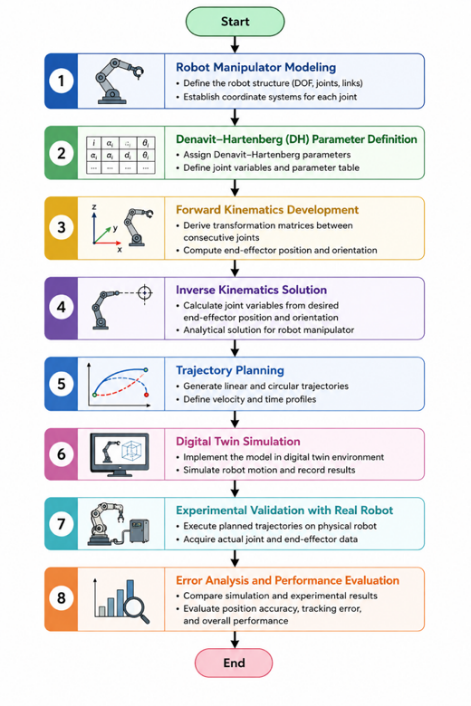
Figure 1. Flowchart illustrating the overall research methodology
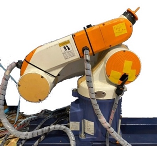
Figure 2. Collaborative Robots 
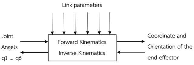
Figure 3. Forward and Inverse Kinematic
Denavit–Hartenberg (DH) Notation
The kinematic equations of the Denso VS-6577 manipulator are formulated using the Denavit–Hartenberg (DH) convention, which provides a systematic approach for modeling serial robotic manipulators. This method describes the spatial relationship between two consecutive links through a homogeneous transformation matrix that defines both the position and orientation of one coordinate frame relative to the preceding frame. For a serial manipulator, the pose of frame  relative to frame
  is represented by the homogeneous transformation matrix
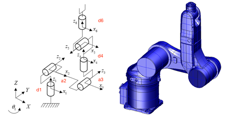
  . This matrix enables the transformation of coordinates from frame to frame and defines the geometric relationship between adjacent joints. The home configuration of the Denso VS-6577 robot and the placement of the DH coordinate frames are shown in Figure 4.
The joint limits of the manipulator are defined as follows 
 According to the DH convention, each link is defined by four parameters: link length
  , link twist
  , link offset
  , and joint angle
  . The homogeneous transformation matrix between two consecutive links is given in Eq. (1). The Denavit–Hartenberg parameters of the Denso VS-6577 manipulator used for deriving the forward and inverse kinematic models are summarized in Table 1. The primary geometric dimensions are specified as.
| 
| (1) |
Table 1. Denavit-Hartenberg Parameter Table
Joint i |

| 
| 
|

| Joint Limit (deg) |
1 | 
| 
| 
| 
| -170, 170 |
2 | 
| 0 | 
| 0 | -100, 135 |
3 | 
| 0 | 
| 
| -119, 169 |
4 | 
| 
| 0 |
| -190, 190 |
5 | 
| 0 | 0 |
| -120, 120 |
6 | 
| 
| 0 | 0 | -360, 360 |

|
Figure 4. The placement of DH parameter of robot
Forward Kinematic
The transformation matrix for each joint is derived from (1) by substituting the corresponding DH parameters specified in Table 1. For the six-degree-of-freedom manipulator, six homogeneous transformation matrices are obtained, representing the relative transformation between consecutive coordinate frames. These matrices are denoted as (2).
| 
| (2) |
| 
|
where  and
and  .
.
The overall homogeneous transformation matrix between the base frame and the end-effector frame is obtained by multiplying the six individual transformation matrices as (3).
| 
| (3) |
Substituting the matrices from (2) into (3) yields the complete forward kinematic model as (4).
| 
| (4) |
In (4),  , denotes the normal vector,
  , denotes the orientation vector,
  , denotes the approach vector, and,
  , denotes the position vector of the end-effector relative to the base coordinate frame. The elements
  are obtained from the symbolic multiplication of the six transformation matrices and are explicitly expressed in (5) to (8).
Inverse Kinematic
The inverse kinematic solution is obtained using an analytical method based on geometric relationships. The joint angles are derived from the end-effector position expressed in Cartesian coordinates  . The resulting equations are given as follows (9) and (16) [26].
| 
| (9) |
| 
| (10) |
| 
| (11) |
| 
| (12) |
| 
| (13) |
| 
| (14) |
| 
| (15) |
| 
| (16) |
The second joint angle is determined as (17) and (22) [26].
The wrist joint angles are computed as (23) and (25) [26].
Since the inverse kinematic formulation may yield multiple solutions, the same end-effector pose can correspond to different joint configurations. To maintain motion continuity, the previous joint configuration was incorporated into the solution selection process, and the configuration with the minimum joint deviation was selected. Among the feasible inverse kinematic solutions, the elbow-up configuration was preferentially selected to maintain trajectory continuity and consistent manipulator posture throughout the motion sequence. In addition, all candidate solutions were evaluated under the predefined joint limit constraints of the manipulator. Singular configurations were considered during trajectory generation and inverse kinematic solution selection. To avoid instability and discontinuous joint motion near singular regions, the manipulator trajectory was constrained within feasible workspace regions away from known singular configurations. These continuity and configuration constraints helped reduce abrupt configuration switching during motion execution. Each inverse kinematic solution was verified by substituting the computed joint angles into the forward kinematic model to ensure that the resulting pose matched the desired end-effector position.
Research Methodology
Application Software and Virtual Simulation
The system integrates MATLAB/Simulink with the Virtual Reality Toolbox (V-Realm) to enable interactive visualization of the kinematic model and end-effector trajectory over time. V-Realm is a three-dimensional virtual simulation environment that extends the capabilities of MATLAB and Simulink with real-time virtual reality graphics. The three-dimensional model of the Denso VS-6577 manipulator, depicted in Figure 5, is connected to the Simulink model via a 3D animation block. This integration enables the visualization of simulated joint angles and control signals as realistic motion in the virtual robot model. Thus, the end-effector trajectory can be analyzed both visually and spatially within the virtual workspace. V-Realm is based on VRML (Virtual Reality Modeling Language) and functions as an interface between MATLAB/Simulink and the three-dimensional virtual model. The joint trajectories are calculated using the inverse kinematic algorithm and transmitted to the simulation environment. The robot then moves from the initial position to the target location in Cartesian coordinates, with the corresponding motion visualized in the virtual environment.
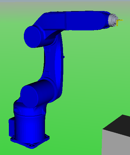
Figure 5. Robot simulation model on Virtual Reality toolbox in home position (right)
Analysis Methodology
An experiment was conducted to validate the forward and inverse kinematic models of the Denso VS-6577. A circular trajectory with a radius of 5 cm in the xy-plane was defined as the reference path to evaluate the kinematic performance and trajectory tracking capability of the robotic system. Before executing the circular trajectory, the manipulator was first moved from the predefined home position to the trajectory starting point through an intermediate transition motion to ensure safe and smooth robot movement. This transition process reduced abrupt joint displacement and minimized sudden directional changes before initiating the circular trajectory. After reaching the starting point, the manipulator executed the circular motion and finally returned to the initial trajectory point to complete the motion cycle.
As shown in Figure 6, the desired trajectory input consisting of time, Cartesian position ( ), and orientation angles (roll, pitch, yaw) was first processed by the analytical inverse kinematic block to generate the corresponding joint variables
  These joint commands were subsequently transmitted to the control system and forward kinematic block for robot motion execution and Cartesian position computation. During operation, the industrial manipulator utilized its built-in servo feedback controller, resulting in a closed-loop trajectory tracking implementation.
The computed Cartesian coordinates obtained from the forward kinematic model were compared with the reference trajectory to evaluate trajectory tracking performance. In addition, the generated robot motion was visualized through the 3D graphical simulation environment, while the root-mean-square errors (RMSE) along the x, y, and z axes were calculated to quantify the differences between the desired and resulting end-effector trajectories.
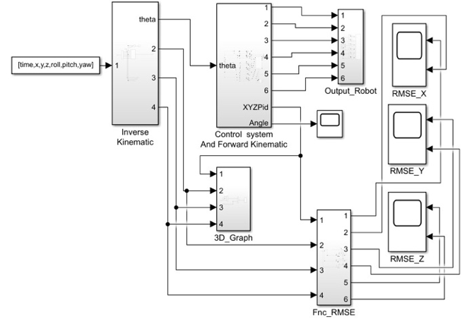
Figure 6. Simulink model for control Robot manipulator
The trajectory data were sampled at a frequency of 1024 Hz during both simulation and physical robot experiments. A total of trajectory points were collected for each experimental trial. To ensure consistency between the virtual simulation and physical robot implementation, identical reference trajectories, trajectory durations, and sampling intervals were applied in both environments. In addition, synchronization between simulation and experimental data acquisition was achieved using the same time-indexed trajectory sequence and Cartesian reference points throughout the validation process. The control system comprises several functional components, including a workspace input block that provides Cartesian coordinate references, an inverse kinematic function block that converts Cartesian coordinates into corresponding joint angles, a control and forward kinematic block, an RMSE evaluation block for calculating positional errors along each axis, and a robot output visualization module for representing manipulator motion.
Joint-space validation was additionally performed by monitoring all computed joint variables  during trajectory execution. The analytical inverse kinematic solutions were constrained by the predefined joint limits of the manipulator, and no joint-limit violations were observed throughout the experimental trajectory. This confirms that the proposed inverse kinematic framework generates physically feasible and continuous robot motion. In the second phase, the joint angles derived from the inverse kinematic function were input into the forward kinematic block to reconstruct the Cartesian position of the end-effector. The reconstructed coordinates were compared with the reference trajectory, and the Root Mean Square Error (RMSE) was computed for each axis to measure positional deviation. This procedure ensures consistency between the forward and inverse kinematic models.
The RMSE evaluation was performed by comparing the reference Cartesian trajectory with the Cartesian coordinates reconstructed from the executed robot motion using the forward kinematic model. Therefore, the computed RMSE values include not only kinematic modeling accuracy but also the effects of the closed-loop servo control system, actuator dynamics, and physical robot execution errors during trajectory tracking. Symbolic derivations were initially performed to obtain the analytical kinematic equations, while numerical computations were used during real-time trajectory execution in MATLAB.
The experiment was conducted under identical conditions for both the virtual simulation model and the real robot system. The initial configuration was defined as the home position:
The end-effector then moved to the starting point of the circular trajectory:
After reaching this position, the manipulator executed a complete 360-degree circular motion in the  -plane before returning to the home position. During the experiment, the output from the inverse kinematic block was transmitted to the control system and visualized within the V-Realm environment, while the reconstructed Cartesian coordinates from the forward kinematic model were evaluated using the RMSE block to determine the accuracy of the kinematic model.
Experimental Result
Results of the Simulation Test
The experimental results are divided into two main sections: the simulation experiment and the real robot experiment. The simulation results evaluate the trajectory performance of the robotic manipulator and examine the consistency between the reference trajectory and the system output. The Cartesian coordinates along the X, Y, and Z axes are analyzed to illustrate the trajectory behavior in each direction, and the Root Mean Square Error (RMSE) is computed to quantify the deviation between the reference and output values. This analysis highlights the importance of the simulation system in predicting and evaluating robot motion prior to real-world implementation.
The experiment consists of three types of motion. The first motion is a point-to-point movement from the home position to the initial point before beginning the circular trajectory. The second motion is circular movement, in which the robot follows a circular path with a radius of 5 cm in the -plane. The third motion is another point-to-point movement, where the robot returns from the final position of the circular path to the home position.
The circular motion is defined by the following equations:
where  cm. The resulting three-dimensional trajectory is shown in Figure 7.
Figure 7 illustrates the three-dimensional trajectory of the robot in the simulation experiment. The motion begins at the home position (0.598, 0, 0.79), moves to the first position of the circular trajectory (0.35, 0, 0.6), performs a complete 360-degree circular motion, and then returns to the home position. As shown in Figure 7, three distinct motion segments can be clearly identified. The first segment corresponds to the point-to-point movement from the home position to the first point. The second segment represents the circular motion with a 5 cm radius. The third segment corresponds to the return movement to the home position.
Two trajectories are presented in Figure 7, the reference trajectory (blue line) and the system output trajectory (red line). A noticeable deviation occurs during the initial transition from the home position to the first point, where errors appear along all three axes. A similar deviation pattern is observed during the return movement to the home position. In contrast, the circular motion phase exhibits significantly smaller deviation.
Figure 8 presents the comparison between the reference and output trajectories along the X-axis. At time 0 s, the robot starts at X = 0.598 m. From 0 to 50 seconds, the robot performs a point-to-point movement toward the first circular position. Between 50 and 410 seconds, the robot follows the circular trajectory defined by the motion equations. Finally, between approximately 450 and 500 seconds, the robot returns to the home position using point-to-point motion. The blue line represents the reference trajectory, while the red line represents the system output. It can be observed that the deviation during point-to-point motion is considerably larger than during circular motion.
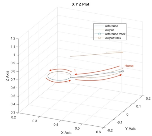
Figure 7. Comparison between the reference trajectory (blue line) and simulated output trajectory (red line) during circular motion execution in the virtual environment
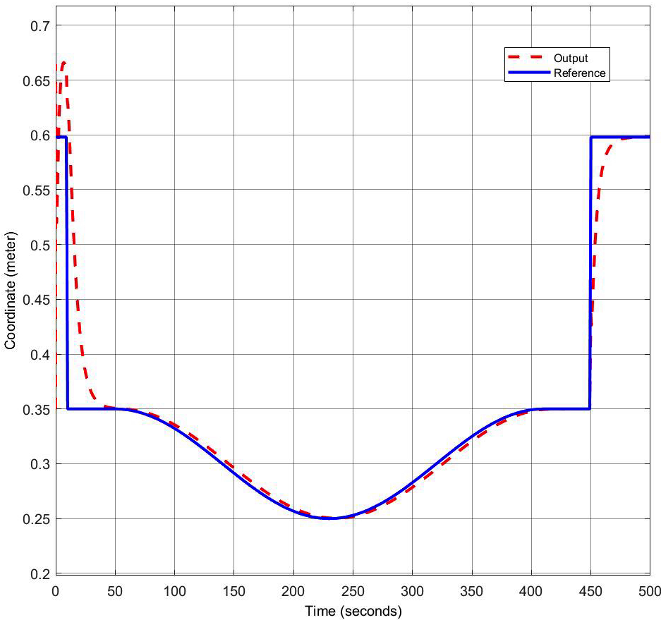
Figure 8. The reference and output path in X coordinate (meter) simulation
Figure 9 shows the RMSE along the X-axis during the simulation experiment. The maximum error in the first point-to-point phase is 0.2151 m. During the circular motion phase, the RMSE significantly decreases to 0.00185 m (1.85 mm), which is consistent with the trajectory comparison shown in Figure 8. In the third phase, the RMSE increases again to 0.2046 m. These results indicate that motion governed by the circular trajectory equation results in substantially lower error compared to point-to-point motion.
Figure 10 illustrates the reference and output trajectories along the Y-axis. Because the trajectory follows a circular path centered at the Y-axis origin, the Y-coordinate oscillates between positive and negative values. The end-effector moves from Y = 0 to approximately +0.035 m and −0.035 m before returning to Y = 0. The output trajectory closely follows the reference; however, a slight phase delay can be observed throughout the circular motion phase.
The slight phase delay observed along the y-axis was primarily attributed to the tuning characteristics of the PID-based servo control system used in the industrial manipulator. During trajectory execution, the controller response introduced a small temporal lag between the reference trajectory and the actual robot motion, particularly during continuous circular movement and directional transitions. This behavior was mainly related to the proportional–integral–derivative gain settings, actuator response dynamics, and acceleration/deceleration characteristics of the closed-loop control system rather than inaccuracies in the analytical kinematic model itself.
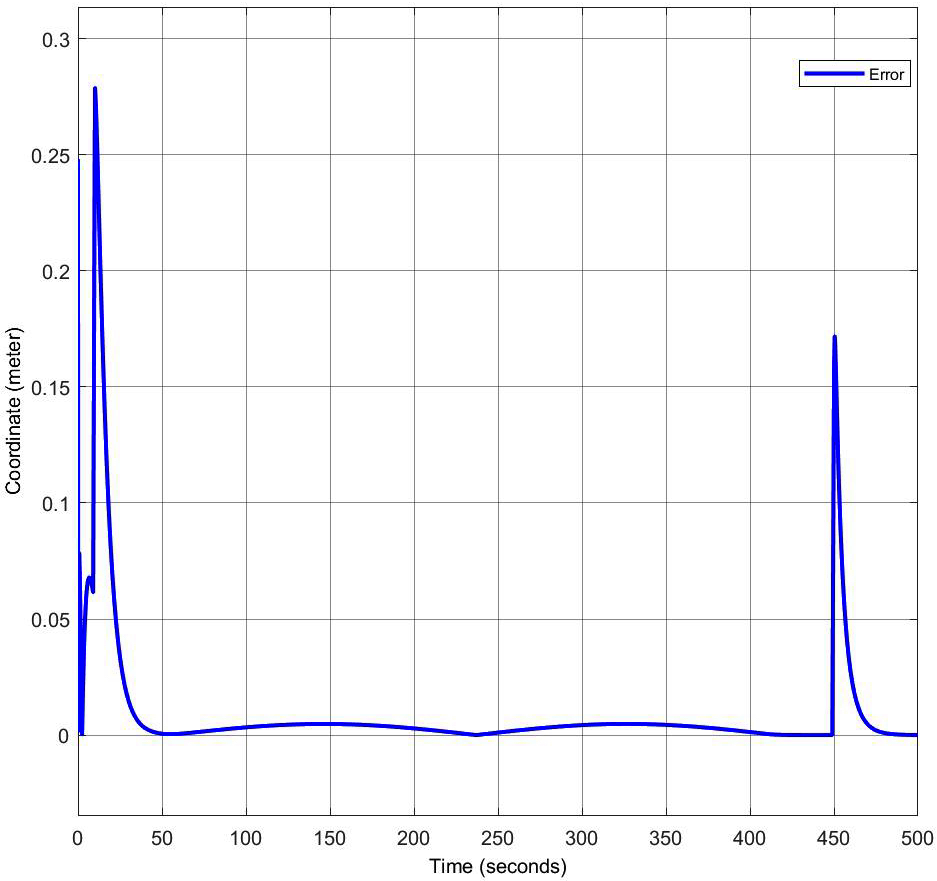
Figure 9. RMSE Along the X-Axis in Simulation
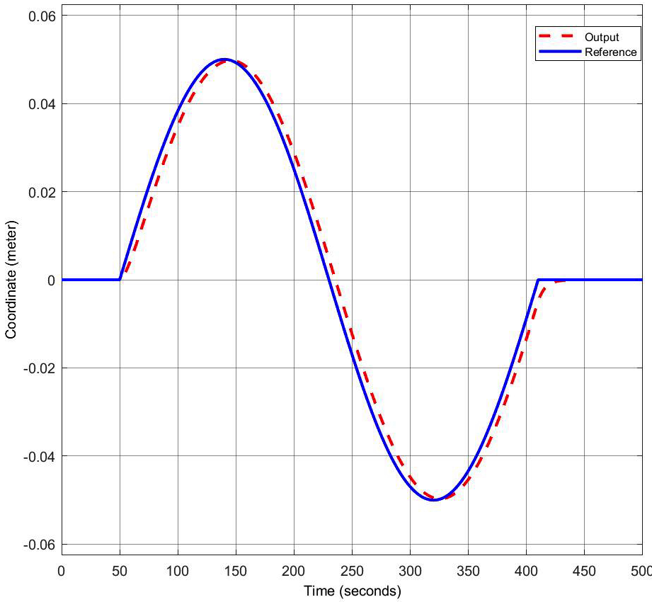
Figure 10. The reference and system output path in Y coordinate (meter) simulation
Figure 11 presents the RMSE in the Y-axis. The maximum Y-axis error is 0.00049 m (0.49 mm). The error increases as the end-effector moves away from Y = 0 and decreases when passing through Y = 0 again. Compared to the X-axis error, the Y-axis deviation remains relatively small throughout the motion. Figure 12 shows the trajectory comparison along the Z-axis. During the initial point-to-point phase, the output trajectory deviates significantly from the reference. In the second phase, when the robot follows the circular motion equation, the output trajectory closely matches the reference. In the third phase, similar deviation patterns reappear, consistent with those observed in the X and Y axes.
Figure 13 presents the RMSE in the Z-axis. The maximum error of 0.27 m occurs during the first point-to-point phase. The error decreases substantially during the circular motion phase and increases again during the final point-to-point movement before returning to the home position. The error characteristics in the Z-axis follow a pattern similar to that observed in the X-axis. Finally, Figure 14 shows the angular displacement of each joint throughout the entire simulation period. The robot begins at the home configuration (0.598, 0, 0.79, 0°, 90°, 0°), moves to the first circular position (0.35, 0, 0.6, 0°, 180°, 0°), performs a full 360-degree circular motion with a 5 cm radius, and then returns to the home position. The joint displacement curves demonstrate smooth variation during the circular motion phase and more abrupt transitions during the point-to-point phases.
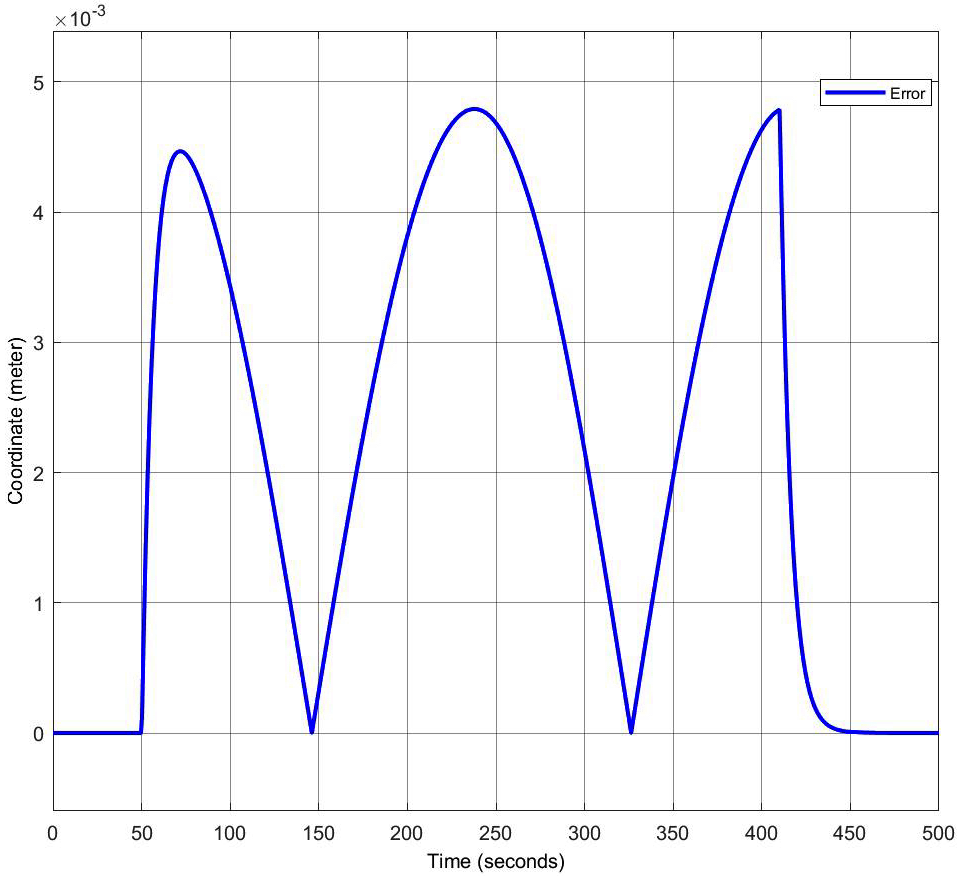
Figure 11. The RMSE in Y coordinate (meter) simulation
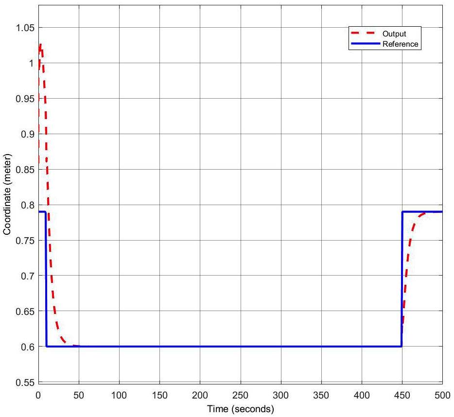
Figure 12. The reference and system output path in Z coordinate (meter) simulation
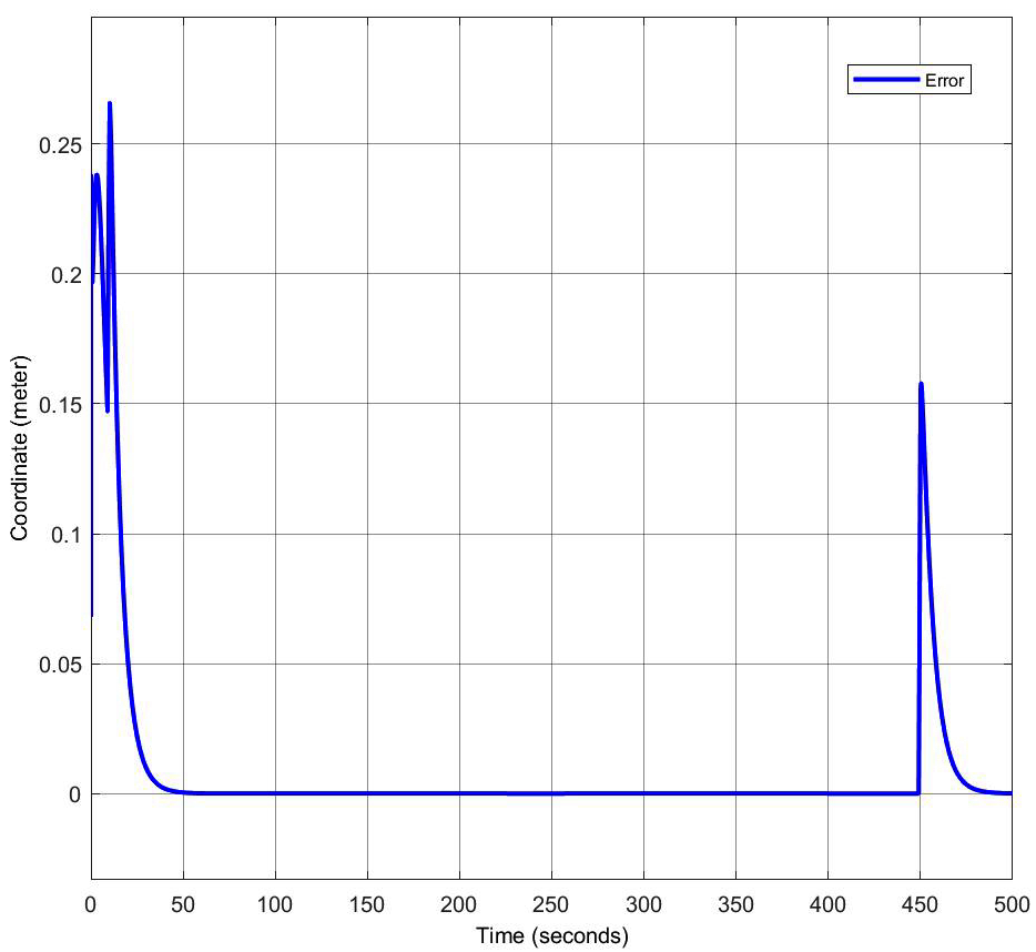
Figure 13. The RMSE in Z coordinate (meter) simulation
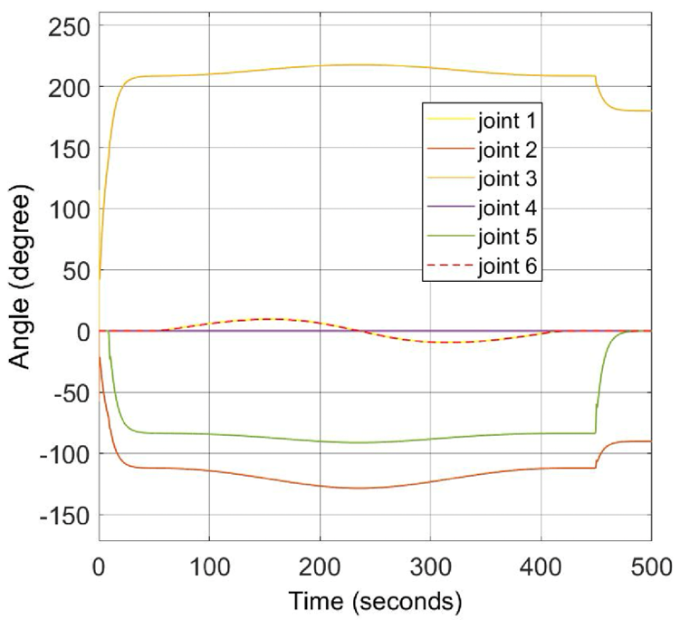
Figure 14. The angular displacement of each joint of robot simulation
Real Robot Test Results
After completing the simulation trials and obtaining the error values for each axis, the next phase involved experimental validation using the actual robotic system. This stage was conducted to implement and verify the kinematic model, which had previously been validated in simulation, under real operating conditions. The trajectory of the end-effector in the real robot experiment was designed to replicate the same circular path with a radius of 5 cm in the -plane, consistent with the simulation setup. The resulting three-dimensional trajectory is shown in Figure 15. The first phase corresponds to the point-to-point movement from the home position to the first point of the circular trajectory, where a relatively large error is observed. The second phase involves circular motion from position 1, completing a full 360-degree revolution and returning to the starting point of the circle. The third phase corresponds to the point-to-point return movement from position 1 back to the home position. The error pattern observed in the real robot experiment is consistent with the behavior identified in the simulation results.
Figure 15 presents the 3D trajectory of the real robot experiment. The red line represents the reference circular trajectory with a radius of 5 cm, while the blue line indicates the measured output trajectory of the robot end-effector. A deviation between the reference and actual trajectories is observed. Similar to the simulation results, the overall motion can be divided into three distinct phases. Figure 16 shows the comparison between the reference and output trajectories along the X-axis. The red line denotes the reference trajectory, while the blue line represents the measured output. The motion begins at the home position (X = 0.598 m), moves to the first circular position at 22.465 s, follows the circular trajectory until 391.331 s, and finally returns to the home position at 430.645 s. The trajectory profile clearly reflects the three motion phases described earlier.
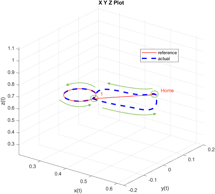
Figure 15. Comparison between the reference trajectory (blue line) and experimentally measured output trajectory (red line) during physical robot trajectory execution
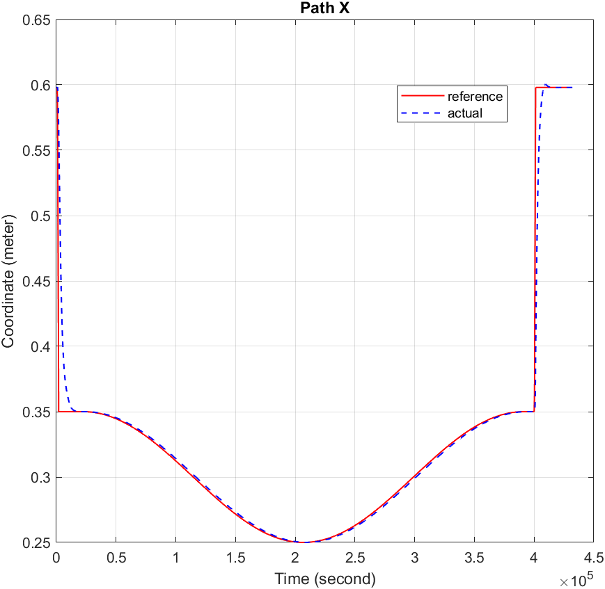
Figure 16. The reference and output path in X coordinate (meter) of Real robot
Figure 17 illustrates the RMSE along the X-axis. The maximum X-axis error of 0.22 m (22 cm) occurs during the initial point-to-point phase (0–22.465 s). During the circular motion phase (22.465–391.331 s), the RMSE significantly decreases to 0.003125 m (3.125 mm). When the robot returns to the home position (391.331–430.645 s), the error increases again, showing behavior similar to the first phase. These results confirm that point-to-point transitions produce substantially larger deviations than circular motion.
Figure 18 illustrates the Y-axis trajectory tracking performance of a real robot, where the red solid line represents the reference (desired) path and the blue dashed line represents the actual output path. The motion follows a smooth sinusoidal-like profile, increasing from zero to a positive peak, then decreasing to a negative minimum before returning to zero. The close overlap between the reference and actual curves indicates that the control system achieves high tracking accuracy with minimal error and stable dynamic response throughout the operation.
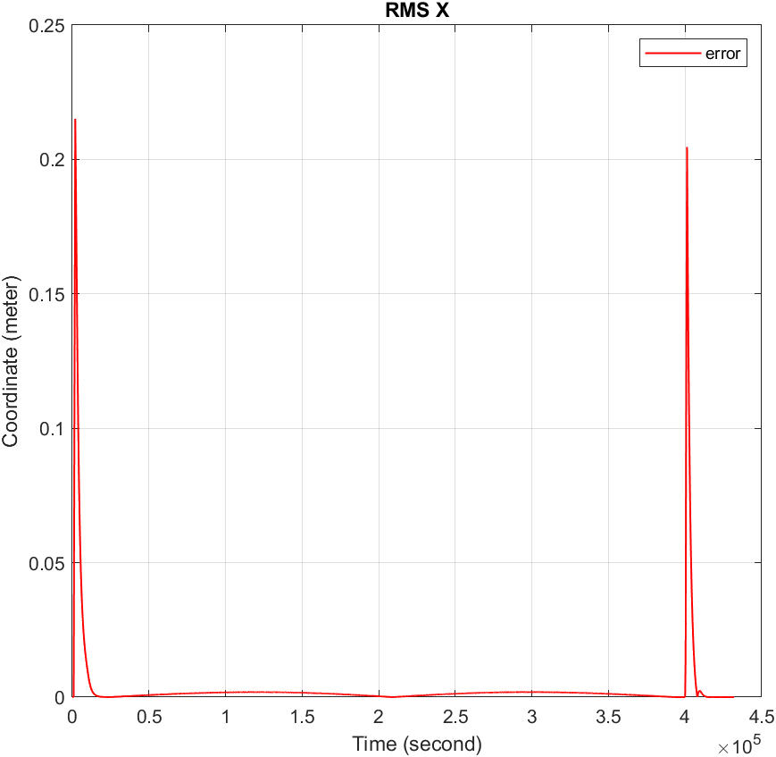
Figure 17. The RMSE in X coordinate (meter) of Real robot
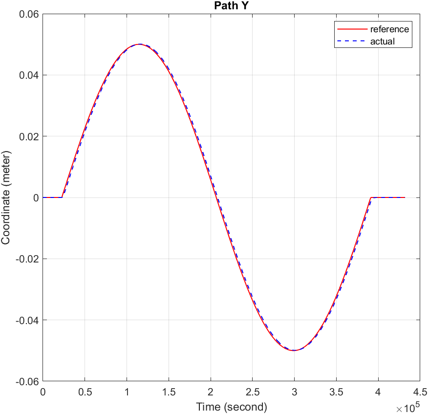
Figure 18. The reference and output path in Y coordinate (meter) of Real robot
Figure 19 shows the RMSE in the Y-axis across the three motion intervals (0–22.465 s, 22.465–391.331 s, and 391.331–430.645 s). The maximum Y-axis error is 0.00131879 m (1.31879 mm), and the minimum error is 3.5e−07 m (0.00035 mm). The error magnitude remains relatively small during the circular motion phase, demonstrating accurate trajectory tracking along the Y-axis.
Figure 20 illustrates the reference and output trajectories along the Z-axis. The robot starts at Z = 0.79 m (home position), moves to Z = 0.6 m at the first circular position (22.465 s), maintains approximately Z = 0.6 m during the circular motion phase (up to 391.331 s), and then returns to Z = 0.79 m at 430.645 s.
During circular motion, the Z-axis reference remained constant because the trajectory was designed in the XY plane only. However, minor fluctuations were observed in the Z-axis output. These variations are relatively small and remain within the acceptable tolerance range of the robot system. The fluctuations are mainly caused by mechanical vibration, sensor noise, joint backlash, and coupling effects between robot joints. Therefore, they do not significantly affect the overall trajectory-tracking performance.
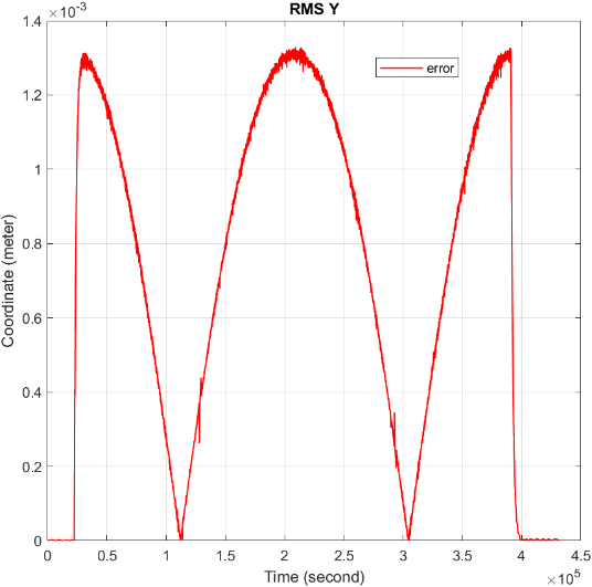
Figure 19. The RMSE in Y coordinate (meter) of Real robot
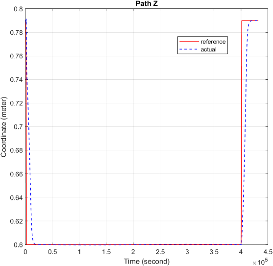
Figure 20. The reference and output path in Z coordinate (meter) of Real robot
Figure 21 presents the RMSE along the Z-axis. The maximum error of 0.17 m occurs during the first point-to-point phase. During the circular motion phase, the RMSE decreases significantly to 8.91e−5 m (0.0891 mm). In the third phase, the error increases again to 0.189 m during the return movement. The error characteristics in the third phase are similar to those in the first phase, as both involve point-to-point transitions.
Finally, Figure 22 shows the angular displacement of each joint throughout the entire real robot experiment. The robot begins at the home configuration (0.598, 0, 0.79, 0°, 90°, 0°), moves to the first circular position (0.35, 0, 0.6, 0°, 180°, 0°), performs a full 360-degree circular motion, and returns to the home position. The joint angle profiles indicate smooth variation during the circular phase and more abrupt transitions during the point-to-point phases, consistent with the simulation results.
Small abrupt changes are observed at the transitions between motion phases, mainly due to sudden changes in velocity and acceleration requirements. These discontinuities can increase transient tracking error and contribute to slight overshoot in the joint responses, especially in the real robot system where actuator dynamics and mechanical backlash are present.
The difference in time duration between the simulation and physical robot experiments was primarily caused by variations in trajectory execution speed and servo response characteristics between the virtual environment and the physical robotic system. Although identical Cartesian reference trajectories and trajectory sequences were applied in both implementations, the actual execution timing of the industrial manipulator was influenced by controller interpolation, actuator acceleration/deceleration limits, and closed-loop servo dynamics. Consequently, slight differences in the overall motion duration were observed between the simulation and real robot experiments.
The initial manipulator posture was configured with  to establish a consistent elbow-up configuration before trajectory execution. This predefined starting posture ensured smooth trajectory initialization, maintained motion continuity, and reduced abrupt configuration changes during the transition and circular motion phases. Although the joint trajectories depended on the selected initial configuration, all computed joint angles shown in Figure 13 and Figure 21 remained within the allowable physical joint limits of the manipulator throughout the entire experimental sequence.
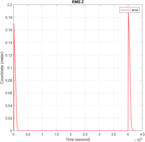
Figure 21. The RMSE in Z coordinate (meter) of Real robot
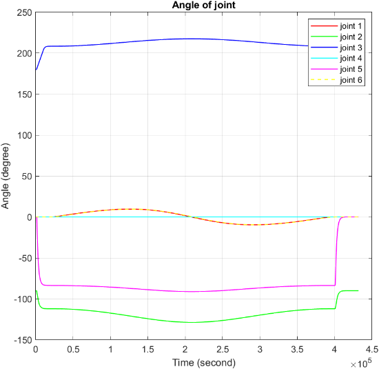
Figure 22. The angular displacement of each joint of Real robot
Table 2 presents the quantitative comparison of the RMSE values obtained from the simulation and physical robot experiments along the x, y, and z axes. The results demonstrate close agreement between the virtual simulation and physical robot implementations. Although small discrepancies were observed, particularly along the x- and z-axes, the overall RMSE values confirm the effectiveness of the proposed analytical kinematic framework for trajectory tracking applications. The remaining differences are primarily attributed to actuator dynamics, servo response delays, mechanical backlash, and modeling uncertainties not included in the ideal kinematic formulation.
Larger point-to-point deviations were primarily observed during transitional movements, particularly when the manipulator changed direction before entering or exiting the circular trajectory. These deviations were mainly attributed to transient servo response dynamics, actuator lag, and abrupt changes in joint velocity and acceleration during trajectory transitions. In addition, minor discrepancies between the analytical kinematic model and the physical robotic system, including mechanical backlash, joint compliance, and DH parameter calibration inaccuracies, also contributed to the observed tracking errors. Although the analytical kinematic framework provided accurate trajectory generation under ideal conditions, the physical robot execution was additionally influenced by closed-loop control response and dynamic constraints not explicitly modeled in the kinematic formulation.
The RMSE values were computed point-by-point over the complete trajectory using all sampled Cartesian data obtained during both the transition and circular motion phases. The calculation was performed by comparing the reference Cartesian coordinates with the reconstructed Cartesian positions generated from the simulation and physical robot experiments. The reported RMSE values represent the root-mean-square average tracking error along each Cartesian axis rather than the maximum instantaneous or peak error during trajectory execution.
The experimental results revealed asymmetric trajectory tracking errors among the Cartesian axes, where the x and z axes exhibited larger point-to-point deviations compared with the y axis. This asymmetry was primarily attributed to the mechanical structure and dynamic characteristics of the articulated manipulator. In particular, motion along the x- and z-directions involved greater shoulder and elbow joint movement, making these axes more sensitive to actuator dynamics, joint compliance, and accumulated kinematic parameter inaccuracies. Furthermore, the z-axis was additionally influenced by gravitational loading and vertical joint deflection effects during trajectory execution. Dynamic effects such as actuator acceleration/deceleration response, servo lag, and inertial coupling between joints also contributed to the observed trajectory deviations, particularly during transitional movements and directional changes. In contrast, the y-axis motion remained relatively stable and less affected by gravitational and dynamic coupling effects, resulting in significantly lower tracking errors.
The experiments were repeated multiple times under the same operating conditions to evaluate the repeatability of the proposed system. The obtained results showed consistent trajectory tracking performance with only minor variations between trials. Therefore, the presented results are considered representative of the typical performance of the robot system.
Table 2. The maximum RMSE values.
Axis | Simulation RMSE (mm) | Experimental RMSE (mm) |
X | 1.85 | 3.125 |
Y | 0.49 | 1.318 |
Z | 0.054 | 0.089 |
CONCLUSION
This study presented a virtual-to-real kinematic modeling and trajectory validation framework for the Denso VS-6577 industrial robotic manipulator. The proposed framework integrated analytical forward and inverse kinematic modeling, MATLAB-based graphical simulation, and physical robot experimentation to evaluate trajectory consistency between simulated and real robotic environments. Experimental results demonstrated satisfactory trajectory tracking performance in both simulation and real robot implementation. During circular motion, the real robot achieved an RMSE of 3.125 mm along the X-axis compared to 1.85 mm in simulation. Although measurable tracking errors were observed due to mechanical backlash, sensor noise, actuator response delay, and unmodeled dynamic effects, the robotic system maintained consistent trajectory tracking behavior throughout the experimental motions. These results confirm the effectiveness of the proposed framework for practical robotic trajectory evaluation and industrial robotic applications. Larger trajectory tracking errors were observed during point-to-point transitional movements because of sudden changes in velocity and acceleration together with actuator and mechanical limitations in the physical robotic system. Nevertheless, the observed errors remained within a practically acceptable range for moderate-accuracy industrial and educational robotic applications where ultra-high precision is not required. The results also indicate that simulation-based trajectory validation can reasonably represent the overall behavior of the physical manipulator despite unavoidable discrepancies between the analytical model and real-world robotic dynamics. This study has several limitations, including the absence of detailed dynamic modeling, limited payload evaluation, and the use of simplified trajectory patterns. Future work will therefore focus on improving robot tracking performance through the integration of dynamic compensation techniques and advanced control approaches such as adaptive control, robust control, and model predictive control (MPC). Additional investigations involving varying payload conditions, more complex robotic trajectories, and trajectory optimization methods will also be conducted to further evaluate the robustness and practical applicability of the proposed robotic framework. The validated virtual-to-real framework demonstrates strong potential for practical industrial automation tasks including robotic assembly, pick-and-place operations, material handling, and welding applications requiring reliable trajectory tracking performance. In addition, the developed kinematic models, trajectory generation procedures, and simulation framework can support reproducibility and future adaptation for related robotic manipulators and robotic trajectory tracking research.
DECLARATION
Acknowledgement
The author would like to express sincere gratitude to Mrs. Chanthana Khawlaor and Mr. Surasarit Khawlaor for their continuous financial support of this research. The author also extends appreciation to Assoc. Prof. Dr. Phichitphon Chotikunnan for his valuable guidance, constructive suggestions, and for kindly reviewing the preliminary versions of the manuscript.
REFERENCES
- M. Y. Alwardat and H. M. Alwan, “Forward and inverse kinematics of a 6-DOF robotic manipulator with a prismatic joint using MATLAB robotics toolbox,” International Journal of Advanced Technology and Engineering Exploration, vol. 11, no. 117, pp. 1096–1110, 2024, https://doi.org/10.19101/IJATEE.2024.111100210.
- H. D. Salman, M. N. Hamzah, and S. H. Bakhy, “Kinematics analysis and implementation of three degrees of freedom robotic arm by using MATLAB,” The Iraqi Journal for Mechanical and Materials Engineering, vol. 21, no. 2, pp. 118–129, 2021, https://doi.org/10.32852/iqjfmme.v21i2.547.
- X. Zhou, Y. Xian, Y. Chen, T. Chen, L. Yang, S. Chen, and J. Huang, “An improved inverse kinematics solution for 6-DOF robot manipulators with offset wrists,” Robotica, vol. 40, no. 7, pp. 2275–2294, 2022, https://doi.org/10.1017/S0263574721001648.
- Y. Wen and P. Pagilla, “Path-constrained and collision-free optimal trajectory planning for robot manipulators,” IEEE Transactions on Automation Science and Engineering, vol. 20, no. 2, pp. 763–774, 2022, https://doi.org/10.1109/TASE.2022.3169989.
- H. Wang, Z. Zhou, X. Zhong, and Q. Chen, “Singular configuration analysis and singularity avoidance with application in an intelligent robotic manipulator,” Sensors, vol. 22, no. 3, p. 1239, 2022, https://doi.org/10.3390/s22031239.
- N. G. Adar, “Real time control application of the robotic arm using neural network based inverse kinematics solution,” Sakarya University Journal of Science, vol. 25, no. 3, pp. 849–857, 2021, https://doi.org/10.16984/saufenbilder.907312.
- M. Li and L. Qiao, “A review and comparative study of differential evolution algorithms in solving inverse kinematics of mobile manipulator,” Symmetry, vol. 15, no. 5, p. 1080, 2023, https://doi.org/10.3390/sym15051080.
- B. Wu, X. Wu, N. Hui, and X. Han, “Trajectory planning and singularity avoidance algorithm for robotic arm obstacle avoidance based on an improved fast marching tree,” Applied Sciences, vol. 14, no. 8, p. 3241, 2024, https://doi.org/10.3390/app14083241.
- J. Villalobos, I. Y. Sanchez, and F. Martell, “Singularity analysis and complete methods to compute the inverse kinematics for a 6-DOF UR/TM-type robot,” Robotics, vol. 11, no. 6, p. 137, 2022, https://doi.org/10.3390/robotics11060137.
- Q. Fan, Z. Gong, S. Zhang, B. Tao, Z. Yin, and H. Ding, “A vision-based fast base frame calibration method for coordinated mobile manipulators,” Robotics and Computer-Integrated Manufacturing, vol. 68, p. 102078, 2021, https://doi.org/10.1016/j.rcim.2020.102078.
- V. Lakshmi Narayanan, J. Narayan, H. Gritli, and S. K. Dwivedy, “A decade of inverse kinematics methods for serial manipulators: A systematic review,” Journal of Field Robotics, vol. 43, no. 1, pp. 184–229, 2026, https://doi.org/10.1002/rob.70014.
- W. He, P. Zhang, K. Guo, J. Sun, V. Sivalingam, and X. Huang, “Kinematic calibration and compensation of industrial robots based on extended joint space,” IEEE Access, vol. 11, pp. 109331–109340, 2023, https://doi.org/10.1109/ACCESS.2023.3322569.
- T. Chen, W. Yang, S. Li, and X. Luo, “An adaptive p-norms-based kinematic calibration model for industrial robot positioning accuracy promotion,” IEEE Transactions on Systems, Man, and Cybernetics: Systems, vol. 55, no. 5, pp. 2937–2949, 2025, https://doi.org/10.1109/TSMC.2025.3535783.
- A. R. Firdaus, C. R. Soru, and H. Soebhakti, “Dynamic modeling and PID control of a 6-DOF robotic arm using ROS and Gazebo,” Journal of Applied Electrical Engineering, vol. 9, no. 2, pp. 141–147, 2025, https://doi.org/10.30871/jaee.v9i2.11027.
- D. Ionescu, A. Filipescu, G. Simion, and A. Filipescu, “Internet of Things-cloud control of a robotic cell based on inverse kinematics, hardware-in-the-loop, digital twin, and Industry 4.0/5.0,” Sensors, vol. 25, no. 6, p. 1821, 2025, https://doi.org/10.3390/s25061821.
- M. Elsisi, K. Mahmoud, M. Lehtonen, and M. M. Darwish, “An improved neural network algorithm to efficiently track various trajectories of robot manipulator arms,” IEEE Access, vol. 9, pp. 11911–11920, 2021, https://doi.org/10.1109/ACCESS.2021.3051807.
- C. Li, P. Zheng, S. Li, Y. Pang, and C. K. Lee, “AR-assisted digital twin-enabled robot collaborative manufacturing system with human-in-the-loop,” Robotics and Computer-Integrated Manufacturing, vol. 76, p. 102321, 2022, https://doi.org/10.1016/j.rcim.2022.102321.
- A. Bonci, F. Gaudeni, M. C. Giannini, and S. Longhi, “Robot operating system 2 (ROS2)-based frameworks for increasing robot autonomy: A survey,” Applied Sciences, vol. 13, no. 23, p. 12796, 2023, https://doi.org/10.3390/app132312796.
- S. Bratchikov, A. Abdullin, G. L. Demidova, and D. V. Lukichev, “Development of digital twin for robotic arm,” in Proceedings of the 2021 IEEE 19th International Power Electronics and Motion Control Conference (PEMC), pp. 717–723, 2021, https://doi.org/10.1109/PEMC48073.2021.9432535.
- H. Li, X. He, Y. Wu, G. Liu, H. Wang, X. Wen, and L. Li, “Digital twin and AI-driven robotic embodied control system: A novel adaptive learning and decision optimization method,” Robotics and Computer-Integrated Manufacturing, vol. 98, p. 103138, 2026, https://doi.org/10.1016/j.rcim.2025.103138.
- G. Singh and V. K. Banga, “Kinematics and trajectory planning analysis based on hybrid optimization algorithms for industrial robotic manipulators,” Soft Computing, vol. 26, pp. 11339–11372, 2022, https://doi.org/10.1007/s00500-022-07423-y.
- Z. Liang, P. Quan, S. Di, and Z. Huang, “Inverse kinematics optimization for redundant manipulators using motion-level factor,” Mathematics, vol. 13, no. 4, p. 624, 2025, https://doi.org/10.3390/math13040624.
- N. Singh, V. K. Tewari, P. K. Biswas, L. K. Dhruw, R. Ranjan, and A. Ranjan, “Optimizing cotton-picking robotic manipulator and inverse kinematics modeling using evolutionary algorithm-assisted artificial neural network,” Journal of Field Robotics, vol. 41, no. 7, pp. 2322–2342, 2024, https://doi.org/10.1002/rob.22247.
- A. Calzada-Garcia, J. G. Victores, F. J. Naranjo-Campos, and C. Balaguer, “A review on inverse kinematics, control and planning for robotic manipulators with and without obstacles via deep neural networks,” Algorithms, vol. 18, no. 1, p. 23, 2025, https://doi.org/10.3390/a18010023.
- S. Zhang, Q. Xia, M. Chen, and S. Cheng, “Multi-objective optimal trajectory planning for robotic arms using deep reinforcement learning,” Sensors, vol. 23, no. 13, p. 5974, 2023, https://doi.org/10.3390/s23135974.
- S. Li, D. Chen, and J. Wang, “An optimal singularity-free motion planning method for a 6-DOF parallel manipulator,” Industrial Robot: The International Journal of Robotics Research and Application, vol. 48, no. 2, pp. 290–299, 2021, https://doi.org/10.1108/IR-04-2020-0079.
- A. Sharkawy and S. Khairullah, “Forward and inverse kinematics solution of a 3-DOF articulated robotic manipulator using artificial neural network,” International Journal of Robotics and Control Systems, vol. 3, no. 2, pp. 330–353, 2023, https://doi.org/10.31763/ijrcs.v3i2.1017.
- M. Makulavičius, J. J. Petronienė, E. Šutinys, V. Bučinskas, and A. Dzedzickis, “Industrial robotic setups: Tools and technologies for tracking and analysis in industrial processes,” Applied Sciences, vol. 15, no. 18, p. 10249, 2025, https://doi.org/10.3390/app151810249.
- C. Zhao, Y. Wei, J. Xiao et al., “Inverse kinematics solution and control method of 6-degree-of-freedom manipulator based on deep reinforcement learning,” Scientific Reports, vol. 14, Art. no. 12467, 2024, https://doi.org/10.1038/s41598-024-62948-6.
Wiroj Khawlaor (Kinematic Modeling of 6-DOF Articulated Robot Arm Denso VS 6577)