Grid-Aligned Patchification for Deep Learning-Based Macrophage Detection in Unstained Brightfield Haemocytometer Images

Mohammad Ikhsan 1, Zino Ramdani Suharto 1, Rizal Azis 1, Basari 2

1 Biomedical Engineering, Department of Electrical Engineering, Universitas Indonesia, Depok, West Java, Indonesia

2 Research Center for Biomedical Engineering, Universitas Indonesia, Depok, West Java, Indonesia

1. INTRODUCTION

Cell viability analysis is fundamental to biomedical research, particularly in regenerative medicine, pharmacology, and cell biology [1]. The haemocytometer remains widely used for cell counting due to its simplicity and low cost [2]. However, manual counting is time-consuming (typically 5–10 min per image), subjective, and prone to inter-operator variability, especially when distinguishing live from dead cells based on subtle morphological cues [3]. Trypan-blue staining is a common chemical alternative for viability assessment but is cytotoxic to viable cells, limits downstream reuse of the sample, and introduces its own acquisition and timing variability. Unstained brightfield imaging is preferred whenever the cells must remain viable for subsequent experiments. Recent image-processing approaches have attempted to automate haemocytometer counting, but most rely on traditional thresholding rather than learned feature representations [4][5].

In the last decade, deep learning has transformed biomedical image analysis, achieving state-of-the-art results in various tasks such as cell detection [6], counting [7][8], and segmentation [9]. Object detection models such as Faster R-CNN [10] and the YOLO family [11][12] have been applied to cell detection [13]-[16] and broadly to medical imaging [17]. For example, Sazak and Kotan implemented a YOLO-based detector to detect blood cells with a reported mean Average Precision at IoU 0.50 (mAP50) of ~93% [18]. Likewise, Mask R-CNN [19] has shown strong performance in cell instance segmentation [20][21]. These models often leverage transfer learning from COCO-pretrained [22] backbones such as ResNet [23] to work effectively even with limited biomedical training data [24]-[26]. Generalist cell segmentation tools including Cellpose [27][28] and StarDist [29] offer pretrained models for diverse cell types.

Although recent benchmarks [9],[30] have highlighted the challenge of generalizing across imaging modalities, these models have advanced the field by offering “out-of-the-box” segmentation for diverse images. However, their performance on unlabeled bright-field data, such as haemocytometer images, has been less explored.

First, most cell detection studies use stained specimens [31][32] or fluorescence-labeled images [7],[33] where cells exhibit high contrast. Unstained brightfield microscopy presents a fundamentally harder challenge [21],[34][35]. Macrophages in haemocytometer fields are small (~15-25 pixels at 100x magnification), weakly contrasted, and morphologically similar between live and dead states. Second, few studies systematically evaluate the effect of image preprocessing strategies such as patch-based tiling on small-object detection performance in microscopy, despite tiling being widely used in whole slide image analysis [36]-[39]. Third, the question of whether pretrained generalist models can replace task-specific fine-tuning for haemocytometer images has not been specifically addressed. Recent work on bright-field segmentation shows that even state-of-the-art generalist models fail on unstained bright-field cells unless specifically fine-tuned [40]. In other words, zero-shot application of Cellpose or StarDist to hemocytometer images may yield poor recall and F1 scores.

To our knowledge, no prior benchmark has evaluated live/dead cell detection specifically on unstained brightfield haemocytometer images using a controlled factorial ablation of preprocessing choices against both fine-tuned and zero-shot deployment modes. We hypothesized that structure-aligned patchification, by restoring the object-to-image area ratio that COCO-pretrained detectors expect, would dominate augmentation and model-architecture choices for this task. This paper provides a quantitative test of that hypothesis. We chose the RAW 264.7 macrophage cell line because it is widely used in immunology, inflammation, and pharmacology research, and because it produces the characteristic mix of rounded-live and darker-irregular-dead morphologies that represent the core difficulty of unstained viability assessment.

The research contributions are as follows:

1. Benchmark study: We conduct a comparative benchmark of five cell detection approaches consisting of two-stage detectors (Faster R-CNN, Mask R-CNN), a one-stage detector model (YOLOv11n-Seg) and two generalist models (Cellpose, StarDist) for live/dead macrophage classification in unstained brightfield haemocytometer images. We include both families because each exercises a distinct capability: two-stage detectors trade compute for robustness at extreme scales, one-stage detectors trade backbone depth for speed, and generalist models trade task specificity for zero-shot generalization.
2. Grid-aligned patchification ablation: We systematically evaluate two preprocessing strategies in a 2x2 factorial ablation study demonstrating that using a fixed grid of small patches is the dominant factor for improving detection performance across models.
3. Zero-shot vs fine-tuning comparison: We compare zero-shot application of Cellpose and StarDist against fine-tuned deep detectors on a common class-agnostic F1 metric, quantifying the gap under the "off-the-shelf" deployment scenario that laboratories actually face.
4. Cost-accuracy analysis: We quantify the inference speed, parameter count, and memory footprint of each fine-tuned approach relative to its detection accuracy, identifying an optimal model for edge and real-time deployment, a question not previously addressed for this task.

Together, these results clarify how modern deep learning tools can, or cannot, be applied to unstained haemocytometer assays and guide algorithm selection for this important domain in biomedical research.

2. RELATED WORK

1. Deep Learning for Cell Detection

Object detection frameworks, specifically convolutional neural networks (CNNs), have been widely applied to biomedical cell analysis [6],[17]. Two-stage detectors like Faster R-CNN have been applied to brightfield cell images, often showing high sensitivity and precision [10],[21],[41]. For instance, Moallem et al. report >95% sensitivity and 99% specificity in detecting breast cancer cells amidst white blood cells using Faster R-CNN on brightfield data [41].

Single-stage detectors from the YOLO family are also commonly used due to their speed [11][12]. Recent studies have applied YOLO to blood cell detection, reporting mAP50 of 93-95% on the BCCD dataset [13]-[16]. Wang et al. [25] demonstrated YOLO-based detection of induced pluripotent stem cells in brightfield microscopy images. These models often use transfer learning to achieve high performance with limited labeled data availability, a common occurrence in biomedical data. Transfer learning from COCO-pretrained [22] ResNet [23] backbones has been shown to improve cell segmentation with limited annotations [24],[26].

In addition to detection, instance segmentation approaches like Mask R-CNN [19] have been extended to cells, often by adding attention or morphological refinements [20][21]. Li et al. applied machine learning to fungal cell counting in haemocytometer images, illustrating interest in automated haemocytometer analysis [42].  Meanwhile, Nakarmi et al. recently compared Faster R-CNN, RetinaNet, and YOLOv8 for pathogen detection in brightfield microscopy, highlighting continued advances in microscopy object detection [43].

2. Generalist Cell Segmentation Models

The Cellpose [27] and StarDist [29] algorithms offer pretrained models intended to provide “zero-shot” cell segmentation without custom training across many cell types and imaging modalities. Cellpose [27] learns a generalizable cell segmentation prior from diverse cell morphologies, while StarDist [29] uses star-convex polygons for nucleus/cell detection. Both provide pretrained models applicable across imaging modalities, and recent multimodality benchmarks [9] have evaluated their generalization. However, their performance can degrade on challenging image types. In brightfield microscopy specifically, recent work found that these generalist models struggle [33]-[35]. For example, Cellpose-SAM (Cellpose augmented with Segment Anything model [44]) shows poor accuracy on label-free brightfield cells. When benchmarked on diverse brightfield live cell images, Cellpose and StarDist often score far lower F1 score (sometimes <25%) compared to a dedicated fine-tuned model. This suggests that applying these models without retraining may be insufficient for unstained hemocytometer images, motivating our evaluation of zero-shot versus fine-tuned performance.

3. Patch-Based Strategies for Small Object Detection

Detecting small objects, like cells in microscopy images, is a known challenge for CNN-based detectors [6],[39],[45]. A common remedy is tiling or patchification: dividing high-resolution images into smaller tiles to increase the object-to-image ratio [36],[38]. Unel et al. demonstrated that training on cropped tiles causes small objects to occupy a larger relative area in each patch and reduces early-layer misses [39]. At inference time, overlapping tiles can be merged back to full-image detections. In medical microscopy, similar strategies have shown promise. For example, tile-based extraction has improved malaria parasite cell detection in stained blood smears [37],[46]. Abdurahman et al. [47] showed that tile-based approaches combined with YOLO improve parasite detection in microscopy images.

Those studies primarily address staining variability, whereas our setting is challenged by low contrast in unstained brightfield imagery. The shared methodological insight is the tiling mechanism itself rather than the underlying image-quality challenge. Feature Pyramid Networks (FPN) [48] address multi-scale detection within a single model, but patchification provides a complementary preprocessing-level solution. The interaction between tiling strategies and data augmentation across architectures has not been systematically studied for cell detection in haemocytometer images [49]-[51].

3. METHODS

1. Dataset

The dataset consists of 24 haemocytometer images of RAW 264.7 macrophage cells acquired using an inverted brightfield microscope at 100× magnification (1600×1200 pixels). No staining was applied, so live/dead differentiation relies solely on morphological characteristics. All images were manually annotated at the instance level with polygon-level instance segmentation masks. In total, the dataset contains 6,307 annotated cells, including 4,492 live cells and 1,815 dead cells, corresponding to a dead-cell ratio of 28.8%. Polygon-level annotations enabled both detection-based and segmentation-based model evaluations.

2. Training and Cross-Validation

We employ six-fold stratified cross-validation at the image level. The 24 images were sorted using   snake ordering based on the proportion of dead cells, and then distributed across folds to maintain similar class distributions. This procedure equalizes the dead-cell ratio across folds better than a round-robin pass, and yields six balanced folds with dead-cell ratios ranging from 27.7% to 29.5% (SD = 0.71%). For each fold, 16 images were used for training, 4 for validation, and 4 for testing. All preprocessing, training, and evaluation steps were performed independently within each fold. Furthermore, splitting was performed before any patch extraction to prevent information leakage between training, validation, and test sets.

Class imbalance was not addressed by explicit reweighting during training: the two-stage detector models were trained with the default class-balanced cross-entropy loss used by the reference configuration, and YOLOv11n-Seg uses the focal-loss classification head native to the Ultralytics YOLO codebase [52]. We did not apply class weights, focal-loss tuning, or resampling; a study of these techniques for dead-cell detection is future work.

3. Grid-Aligned Patchification

We use the term patchification to denote structure-aligned tile extraction guided by the imaging protocol, specifically, the 4×4 counting grid of the haemocytometer chamber. This is distinct from content-agnostic approaches such as sliding-window tiling or SAHI, in that each extracted tile corresponds to a semantically meaningful counting region defined by the physical grid rather than to a regular window over the pixel raster. At 100× magnification, cells occupy only ~15–25 pixels in the full-resolution images, well below the COCO small-object threshold of 32×32 pixels. Patchification addresses this scale mismatch by remapping each grid cell to a 256×256 patch, while also preserving the chamber-level spatial semantics required for downstream counting.

Grid-detection pipeline. The automated grid-detection pipeline is fully deterministic with fixed parameters. We (1) enhance contrast with CLAHE (clipLimit = 2.0, tileGridSize = 8×8), (2) apply a Gaussian blur (kernel ), (3) compute Sobel gradients (ksize = 3) in the horizontal and vertical directions, (4) run Canny edge detection (low/high thresholds = 120/240) on each gradient map, (5) apply the standard Hough transform (, accumulator threshold = 300) separately to the horizontal and vertical edge maps, (6) merge collinear detections and cluster line intersections to recover the 5×5 lattice of inner grid lines, and (7) compute a perspective transform that maps each of the 16 grid cells to a 256×256 output patch. A grid detection is considered successful when the pipeline recovers four outer-chamber corners and at least three interior lines in each direction; we call the resulting perspective-warped 256×256 tile a valid square. Timing on the 24 base images (Apple M1, single thread) shows the pipeline runs in 35.7 ± 3.8 ms per image, with Hough transform (25.9 ms) the dominant cost and the 16 perspective warps adding 2.9 ms in aggregate. The pipeline succeeded on all 24 images: 20 images yielded 16 valid squares each; the remaining 4 yielded 12 valid squares because part of the chamber grid lay outside the imaging field of view. Those four images were distributed across four different folds, so no single fold received more than one reduced-yield image.

Boundary-cell handling. Annotation assignment uses a centroid-based rule. For each cell, the polygon coordinates were transformed using the same perspective warp applied to the corresponding image patch. This ensured spatial consistency between the patch image and its associated instance annotations. Each polygon's centroid determines the single grid cell to which the annotation is assigned. Polygons that cross a grid-line boundary are clipped to the grid cell, and the resulting geometry is reduced to its largest component. All clipped polygon coordinates are then transformed by the same 3×3 homography used for the image patch so the annotation-to-patch correspondence is exact. Cells whose centroid lies on a grid line are deterministic ties broken by preferring the lower-row/left-column cell. The extracted patches cover approximately 66% of the original image area, correctly excluding regions outside the counting grid per standard haemocytometer protocol.

Annotation quality control. To mitigate single-annotator bias, a second annotator reviewed every polygon on every image. Disagreements were reconciled before the dataset was finalized. We did not compute a formal inter-rater agreement statistic, and this remains a limitation. A large-scale replication with multiple independent annotators and an inter-annotator reliability study is future work.

Figure 1 illustrates a representative whole-image sample with the detected grid overlay and transformed ground-truth annotations, together with example 256 × 256 patches showing variability in cell density and class composition. Figure 2 presents zoomed examples of annotated live and dead cells. In general, live cells appear brighter, more rounded, and more clearly bounded, whereas dead cells tend to be darker, less regular in shape, and lower in contrast. Figure 3 summarizes the end-to-end methodology.

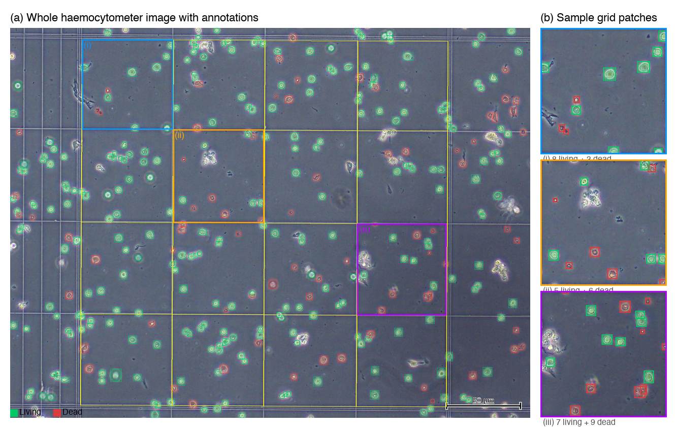
Figure 1. Dataset overview. (a) A whole haemocytometer image (1600x1200) with 4x4 grid overlay (yellow lines) and ground truth annotations (green: living, red: dead). Highlighted regions (i)-(iii) correspond to (b) three sample 256x256 patches showing varying cell densities and class distributions

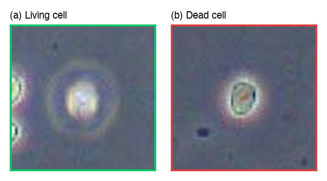
Figure 2. Zoomed views of individual cells with annotations. (a) Living cell: bright, round morphology with well-defined borders. (b) Dead cell: darker appearance with irregular shape and reduced contrast

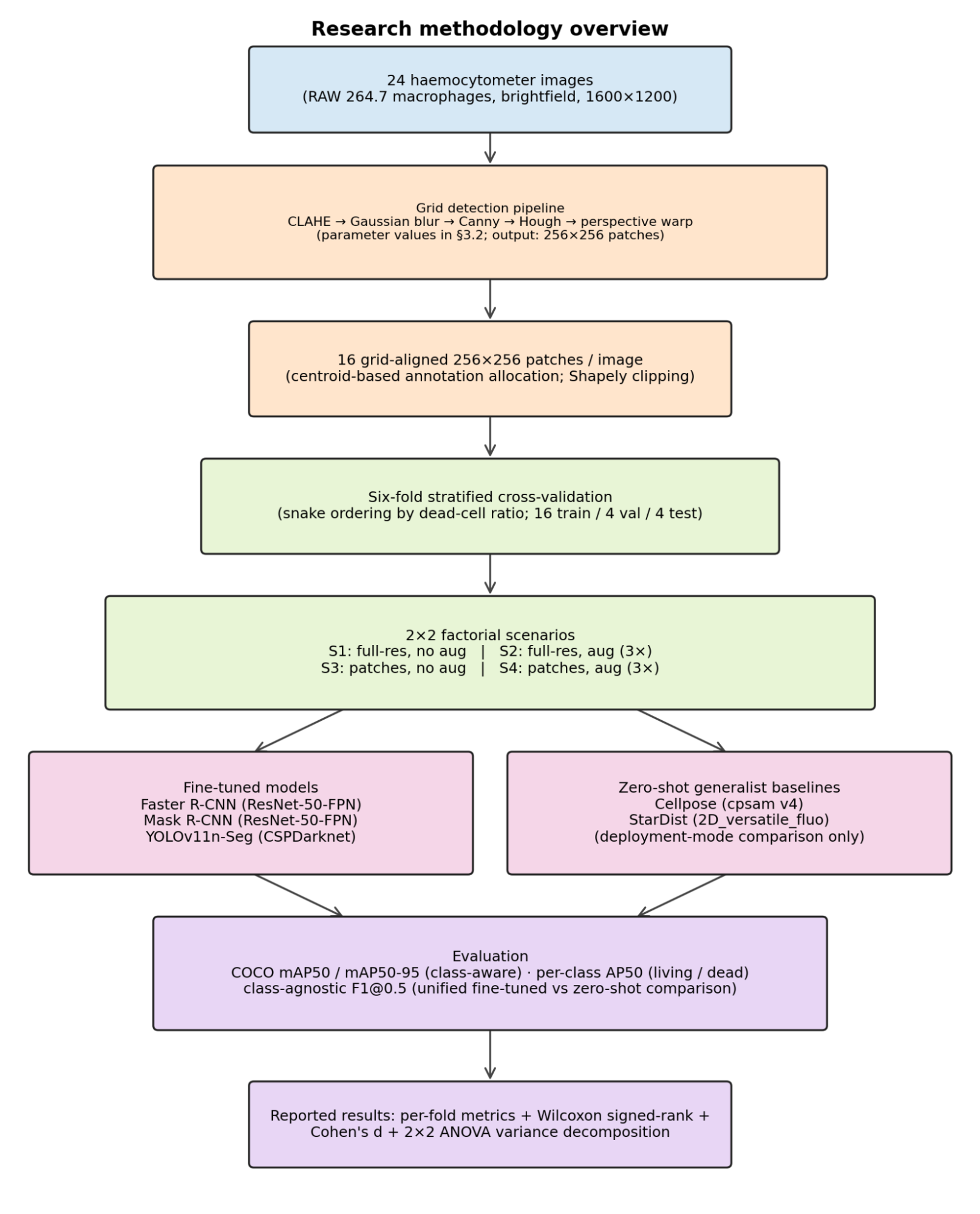
Figure 3. End-to-end research methodology. 24 brightfield haemocytometer images are passed through the deterministic grid-detection pipeline to yield 16 grid-aligned 256×256 patches per image. Fold assignment (six-fold stratified CV with snake ordering by dead-cell ratio) and the 2×2 factorial scenario design precede training. The fine-tuned branch (Faster R-CNN, Mask R-CNN, YOLOv11n-Seg) is evaluated under class-aware COCO mAP. The zero-shot branch (Cellpose, StarDist) is evaluated as a deployment-mode comparison under class-agnostic F1@0.5

4. Experimental Scenarios

We conducted a 2×2 factorial study to evaluate the effects of two preprocessing factors: data augmentation and grid-aligned patchification. This yielded four experimental scenarios summarized in Table 1. We hypothesized that patchification would be the dominant factor because it directly addresses the small-object scale mismatch identified above, while augmentation was expected to yield only modest marginal gains. The 256×256 patch size was chosen because it matches the effective grid-cell extent after perspective warp at 100× magnification and it is an integer multiple of the stride of all three fine-tuned detectors' input pipelines. A patch-size sensitivity study is future work.

Data augmentation was applied only to the training split and used a threefold expansion factor: each training image produced three augmented variants, so the training-set size was tripled while validation and test splits were left unchanged [49],[51]. The augmentation pipeline used horizontal and vertical flips, brightness perturbation of ±15%, Gaussian blur, and additive Gaussian noise. These operations were chosen to match the dominant variability sources in brightfield microscopy acquisition (illumination drift, focus drift, and sensor noise). All geometric transformations were applied in an annotation-consistent manner using polygon transforms, and the random seed was fixed per fold to ensure reproducibility.

Table 1. Experimental Scenario Design (2×2 Factorial)

5. Model Architectures

Five model families were evaluated.

1. Faster R-CNN [10]: Two-stage detector with ResNet-50-FPN backbone, pretrained on COCO. Produces bounding boxes and class labels.
2. Mask R-CNN [19]: Extends Faster R-CNN with a mask prediction head for instance segmentation. Same ResNet-50-FPN backbone and implementation framework for fair comparison.
3. YOLOv11n-Seg [53]: Single-stage detector with instance segmentation capability. The nano variant (2.6M parameters) was selected to reflect a deployment-oriented trade-off between accuracy and computational cost. Also initialized with COCO-pretrained weights.
4. Cellpose [27]: Pretrained generalist cell segmentation model. The cpsam v4 model was used in zero-shot mode without domain-specific fine-tuning.
5. StarDist [29]: Star-convex polygon cell detector. We evaluate the 2D_versatile_fluo (fluorescence) pretrained variant in zero-shot mode without domain-specific fine-tuning.

The first three models were trained to distinguish live and dead cells. In contrast, Cellpose and StarDist were treated as class-agnostic baselines because their pretrained models do not natively predict cell viability categories.

6. Training Configuration

All fine-tuned models were trained on a single NVIDIA A100 GPU using transfer learning from COCO-pretrained weights. Hyperparameters, summarized in Table 2, were fixed a priori from each framework's documented defaults rather than tuned per fold or per architecture. This choice deliberately preserves the controlled-comparison design of the 2×2 factorial experiment and avoids conflating preprocessing effects with tuning effects. Only the training length was governed by per-fold early stopping, which monitored validation mAP50 with a patience length of 20 epochs. Within each fold, the validation split was used for early stopping only, whereas the test split was reserved exclusively for final evaluation. Cellpose was run with the cpsam v4 checkpoint on the cyto channel, and StarDist with the 2D_versatile_fluo pretrained model. Both were applied in zero-shot mode with intensity normalization as their only preprocessing step (no brightfield-specific StarDist variant exists, so the fluorescence model was chosen because its "bright object on dark background" prior most closely matches brightfield contrast).

Table 2. Training Hyperparameters

7. Evaluation Protocol

We use two evaluation tracks that serve complementary purposes.

1. Class-aware protocol for fine-tuned models. Evaluated using the COCO evaluation protocol. Faster R-CNN, Mask R-CNN, and YOLOv11n-Seg are evaluated using the standard COCO protocol via unmodified pycocotools [22]. We report bounding-box mAP50 and mAP50-95 (mean Average Precision at IoU ≥ 0.50 and at the IoU sweep 0.50–0.95 in steps of 0.05), and we break mAP50 down by class (living vs. dead) to assess the viability-classification capability that matters for the downstream counting task.
2. Class-agnostic deployment-mode protocol for zero-shot comparison. Cellpose and StarDist do not predict a viability label in zero-shot mode, so a direct class-aware comparison is not possible. To compare the two groups on a common metric, we collapse both the ground-truth labels and the fine-tuned model's predictions to a single class (“cell”), and report Precision, Recall, and F1 at IoU = 0.50. This merge is a lower bound on the quality gap between the two groups, because the fine-tuned models' class-agnostic F1 can only match or exceed their class-aware F1 (collapsing classes never hurts detection-only accuracy). The gap in class-aware performance is therefore at least as large. We emphasize that this comparison evaluates deployment modes (zero-shot use of published weights) rather than architectural capability. Fine-tuning Cellpose or StarDist on our dataset was deliberately out of scope and is acknowledged as a limitation in the Conclusions.

To compare scenarios and models across folds we use the paired Wilcoxon signed-rank test as the primary non-parametric test, complemented by the paired t-test, both with . For every paired comparison we also report Cohen's d (standardized mean difference for paired samples) and the matched-pairs rank-biserial correlation as effect-size measures. For the 2×2 factorial, we additionally compute  from an ANOVA decomposition to attribute variance across the patchification main effect, the augmentation main effect, the interaction, and the residual.

4. RESULT AND DISCUSSION

1. Detection Performance

Table 3 summarizes bounding-box detection performance across all fine-tuned models and experimental scenarios. The most prominent result is the large and consistent gain obtained from grid-aligned patchification. Moving from full-resolution training (S1) to patchified training (S3) increased mAP50 from 31.4% to 84.6% for Faster R-CNN, from 32.8% to 84.7% for Mask R-CNN, and from 10.1% to 85.1% for YOLOv11n-Seg. Similar gains were observed when augmentation was added (S2 to S4). These gains were statistically significant across folds (p = 0.016, Wilcoxon signed-rank test). As visualized in Figure 4, these improvements are much larger than those obtained from augmentation alone, indicating that patchification is the dominant factor driving detection performance. The same trend is visible at the stricter mAP50-95 threshold in Figure 5, where performance remains low on full-resolution images but rises sharply once patchification is applied.

On full-resolution images (S1 and S2), the two-stage detectors achieved substantially better performance than YOLOv11n-Seg. Faster R-CNN and Mask R-CNN reached approximately 31–33% mAP50, whereas YOLOv11n-Seg remained below 11% mAP50. This result indicates that direct training on whole haemocytometer images leaves the cells too small relative to the image size, especially for a lightweight single-stage detection model. By contrast, after patchification (S3 and S4), all three fine-tuned models converged to a similar mAP50 range of 84.6–86.4%. Thus, the main limitation in the baseline setup was not the detector family itself, but the scale mismatch between the objects and the input image.

Table 3. Bounding Box Detection Performance (mAP, %)

Differences between architectures became more apparent at the stricter mAP50-95 threshold. In both patchified settings, YOLOv11n-Seg achieved the highest localization accuracy, reaching 49.3% in S3 and 51.1% in S4, compared with approximately 45–46% for Faster R-CNN and Mask R-CNN. As shown in Figure 5, this indicates that once the scale problem is corrected, YOLOv11n-Seg not only detects cells reliably but also localizes them more precisely. This advantage is statistically significant on patchified data (), making YOLOv11n-Seg the strongest detector overall under the proposed preprocessing pipeline. In practical terms, this is important because haemocytometer analysis may later be extended beyond counting toward morphology-aware downstream tasks.

Data augmentation alone produced only limited benefit. Comparing S1 and S2, augmentation yielded negligible improvement for Faster R-CNN and Mask R-CNN and even reduced YOLOv11n-Seg performance at full resolution. In contrast, when combined with patchification (S4), augmentation provided a small additional gain over S3, especially for YOLOv11n-Seg. This pattern indicates that augmentation is not a substitute for resolving the scale problem. Instead, its value appears secondary, contingent on whether the detector is already operating at a scale where cell features are visually meaningful.

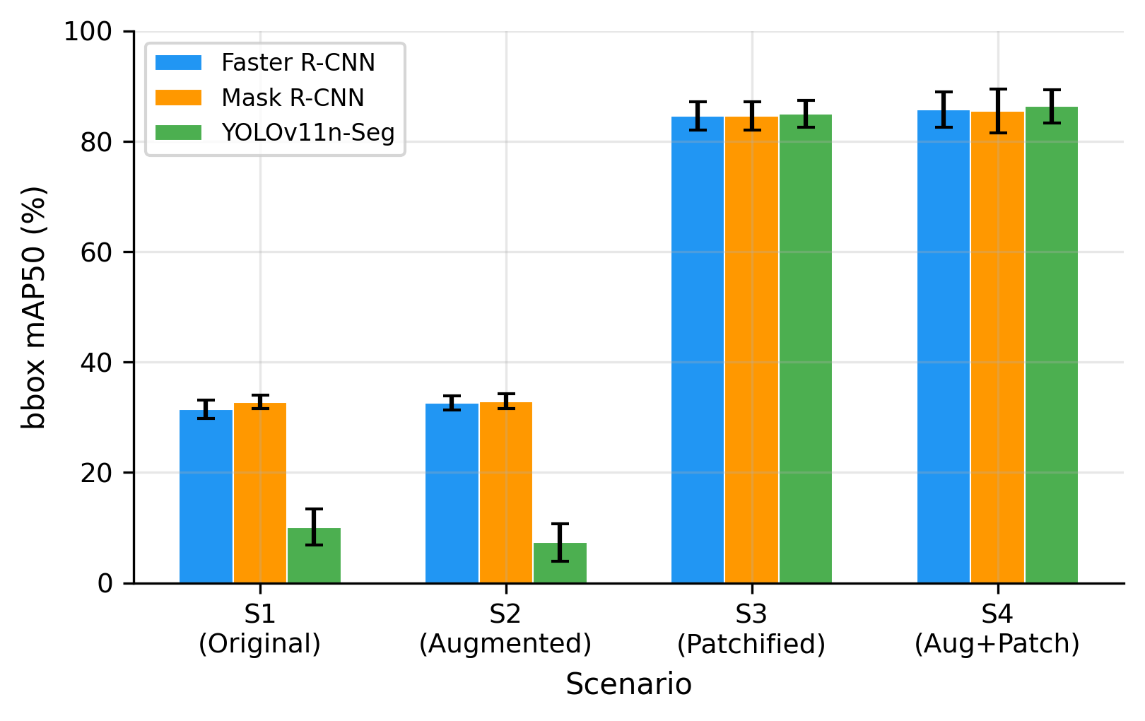
Figure 4. Effect of patchification on detection performance (mAP50) across all scenarios and models. Patchification (S1 to S3, S2 to S4) produces 2.6-8.4x improvements, while augmentation alone (S1 to S2) has minimal effect

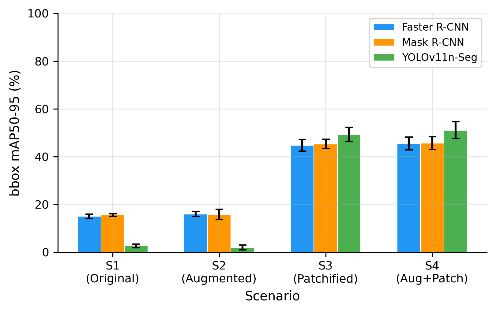
Figure 5. Effect of patchification on stricter mAP50-95. YOLOv11n-Seg achieves the highest mAP50-95 on patchified scenarios, significantly outperforming Faster R-CNN and Mask R-CNN models (p = 0.031)

The factorial trends are summarized more directly in Figure 6, which shows the per-fold distributions across all four scenarios. To quantify the relative contribution of the two factors we run a 2×2 ANOVA and report  on the bounding box mAP50 per model (Table 4). The patchification factor accounts for 99.3%, 99.2%, and 99.4% of the explained variance for Faster R-CNN, Mask R-CNN, and YOLOv11n-Seg respectively. The augmentation main effect is ≤ 0.1% and the patchification × augmentation interaction term is ≤ 0.1% in every case, while the residual is ≤ 1.5%. Grid-aligned extraction transforms cells from small objects (< 1% of image area) to medium-sized objects (~6–10%), bringing them within the effective detection range of all architectures. Although the augmentation main effect is negligible in aggregate, the model-specific interaction pattern is interesting. For Faster R-CNN and Mask R-CNN, augmentation adds a small positive increment once patchification is applied (~+1 mAP50). For YOLOv11n-Seg the interaction is pronounced, augmentation is harmful at full resolution (−2.8 mAP50) but beneficial after patchification (+1.3 mAP50). We interpret this crossover as photometric perturbations erasing already-fragile tiny-object cues on full-resolution images, but providing useful regularization once cells occupy a learnable scale.

Table 4. 2×2 factorial variance decomposition on bounding box mAP50 (, % of explained variance)

Qualitative examples further support the quantitative results. As shown in Figure 7, YOLOv11n-Seg predictions on S4 test patches closely follow the ground-truth annotations in the best-performing fold, with both live and dead cells detected at high confidence. In the worst-performing fold, more missed or misclassified cells are visible, but the model still retains useful detection behavior. These examples are important because they show that the reported improvements are not only numerical but also visually meaningful at the patch level.

Overall, these results support a clear conclusion: patchification is the key enabling factor for accurate cell detection in unstained brightfield haemocytometer images. Once the cells are resized into a more favorable object scale, architectural differences become much smaller at the coarse detection level, and model selection shifts toward efficiency and localization quality rather than raw detectability alone.

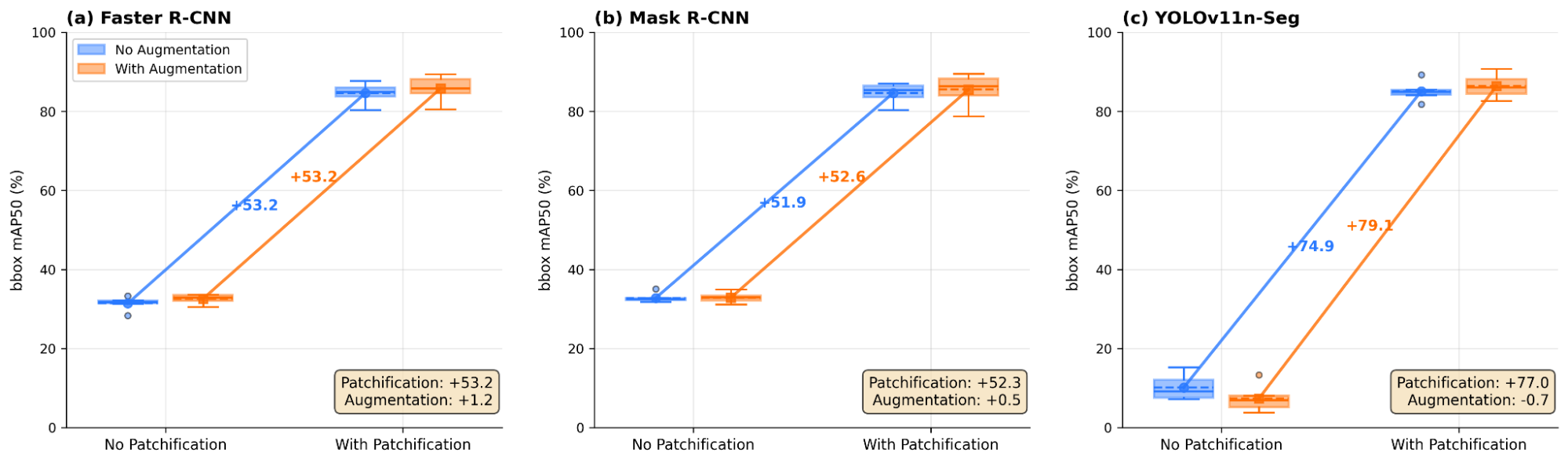
Figure 6. 2x2 factorial ablation of patchification and augmentation for all three models. Box-whisker plots show per-fold distributions. Patchification accounts for >98% of total improvement across all architectures. (a,b) Faster R-CNN and Mask R-CNN  models show consistent augmentation benefit (~+1%). (c) YOLOv11n-Seg exhibits a crossover interaction: augmentation is harmful at full resolution (-2.8%) but beneficial on patches (+1.3%)

2. Instance Segmentation

Table 5 shows that instance-segmentation performance closely tracks the detection results. On the best-performing setup (S4), segmentation mAP50 remained within 1-2 percentage points of bounding-box mAP50 for both Mask R-CNN and YOLOv11n-Seg, indicating that the models were able not only to localize cell instances but also to recover reasonably accurate object shapes. This is notable given the weak contrast and irregular boundaries of unstained brightfield cells.

The close correspondence between detection and segmentation suggests that the benefits of patchification are not limited to coarse localization. Instead, patchification appears to improve the underlying visual representation sufficiently for the models to learn both where the cells are and how their boundaries are shaped. This is relevant for future extensions beyond cell counting, such as morphology-aware analysis or downstream phenotyping tasks.

Table 5. Instance Segmentation Performance (mAP, %)

3. Per-Class Performance

As shown in Table 6, per-class analysis revealed a consistent performance gap between live and dead cells. For each model we report bounding-box AP50 for the two viability classes on the test folds of S4, averaged across all six folds. In the patchified setting, all models achieved substantially higher AP50 for live cells (~93-95%) than for dead cells (~78%), with a gap of roughly 14-16 points. As shown in Figure 8, this pattern persisted across architectures, which suggests that it reflects an intrinsic property of the task rather than a weakness of one specific detector.

The gap is statistically significant across folds for all three architectures: paired one-sided Wilcoxon (live > dead) yields  (the minimum attainable at , with Cohen's  for Faster R-CNN, 3.51 for Mask R-CNN, and 5.08 for YOLOv11n-Seg, all large effects). Two factors likely contribute to this gap. First, the dataset is imbalanced, with live cells outnumbering dead cells (2.5:1 live-to-dead ratio). We did not apply class-weighted or focal-loss re-weighting, so the training signal under-represents dead cells. Second, dead cells appear morphologically less distinct in unstained brightfield images: they are darker, less regular, and often lower in contrast. These characteristics make them intrinsically harder to detect and classify, especially in the full-resolution setting.

Patchification transforms this gap but does not eliminate it: per-class AP50 across all four scenarios shows that dead-cell AP jumps from 25–31% on full-resolution (S1/S2) to 75–79% on patched (S3/S4) for the two-stage detection models, and from 0% to ~78% for YOLOv11n-Seg. A detection-count analysis further reveals that the per-architecture errors are directionally different: on S4, Faster R-CNN and Mask R-CNN both over-predict dead cells (dead prediction/ground-truth count ratios ~1.16 and ~1.19 respectively with false-positive-dominant errors), while YOLOv11n-Seg under-predicts dead cells (ratio ~0.77, false-negative-dominant, missing roughly one in four dead cells on average). This split between FP-biased and FN-biased error modes is consistent with Cellpose/StarDist's similar bimodal behavior in the zero-shot comparison and is a natural target for future class-balanced loss functions.

Table 6. Per-Class Detection AP50 on S4 (Best Scenario, %). The gap is the mean living-minus-dead difference and is statistically significant for all three models (paired Wilcoxon one-sided p = 0.0156; Cohen's d ≥ 3.5, large effect)

Figure 7. Ground truth vs. YOLOv11n-Seg predictions on S4 test patches (green: living, red: dead). Cell counts (L = living, D = dead) shown below each image. (a) Best case patches from Fold 5: predictions closely match ground truth. (b) Worst case patches from Fold 4: more missed or misclassified cells

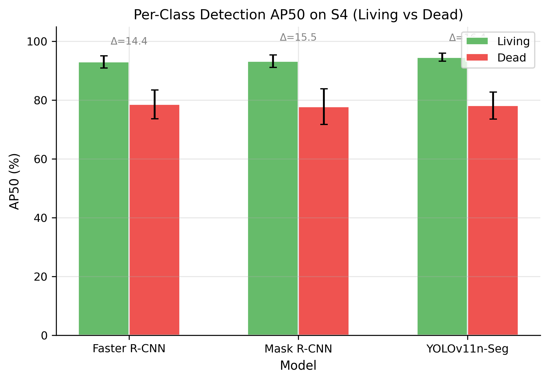
Figure 8. Per-class AP50 across models and scenarios. All architectures show a consistent 14-16 point gap between living and dead cell detection on S4, indicating the gap is morphology-driven

4. Zero-Shot Baseline Comparison

Table 7 compares pretrained generalist models against our fine-tuned models using a unified class-agnostic F1@0.5 metric. For fine-tuned models, we merge living and dead predictions into a single "cell" class and evaluate detection at IoU >= 0.5, enabling direct comparison. Because merging classes can only match or improve detection-only F1 relative to the class-aware case, the reported class-agnostic F1 for fine-tuned models is an upper bound on their class-aware F1, and the 31–33 point gap reported below is therefore a lower bound on the gap one would observe under class-aware evaluation. This section is framed as a deployment-mode comparison: Cellpose and StarDist are used in zero-shot mode with their published weights, as an on-the-shelf lab would use them. Fine-tuning either generalist model on our dataset is out of scope here and is acknowledged as a limitation.

Table 7. Fine-Tuned vs. Zero-Shot Models on S4 (Class-Agnostic F1@0.5, %)

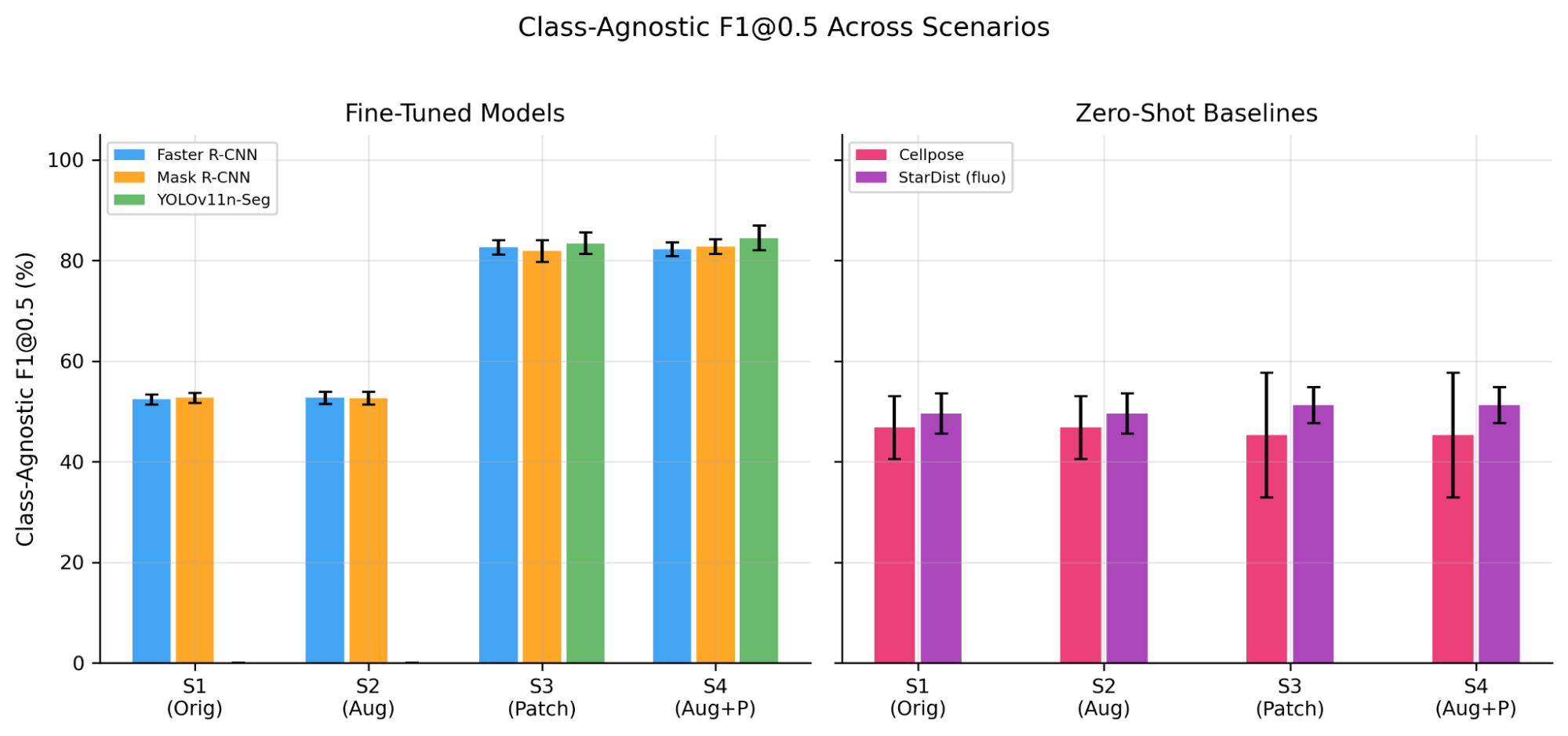
As shown in Figure 9, the best fine-tuned model (YOLOv11n-Seg, 84.4% F1@0.5) outperforms the best zero-shot model (StarDist, 51.2%) by 33.2 percentage points on the same metric. Even the lowest-scoring fine-tuned model (Faster R-CNN, 82.2%) exceeds StarDist by 31 percentage points. All fine-tuned models achieve consistently high recall (~94.9-95.6%), detecting nearly every cell, while differing mainly in precision (72.1-76.2%). In contrast, Cellpose achieves high precision (78.5%) but low recall (32.7%), detecting only one-third of cells, and StarDist shows moderate performance on both axes (58.3% precision, 45.7% recall).

Notably, as shown in Figure 10, patchification has no effect on zero-shot baselines (S1 approximately equal to S3, S2 approximately equal to S4), in stark contrast to the 2.6-8.4x improvement seen with fine-tuned models. This indicates patchification is a training-time benefit, not merely an inference-time preprocessing step. The 31-35 point F1@0.5 gap between fine-tuned and zero-shot models on the same class-agnostic metric demonstrates that unstained brightfield haemocytometer images fall outside the training distribution of current generalist cell segmentation tools. Cellpose's high-precision/low-recall pattern suggests its morphology prior recognizes only the most prototypical cells. StarDist's fluorescence model achieves moderate performance (51.2% F1), likely because the "bright object on dark background" contrast pattern partially matches brightfield imaging. This finding has practical implications: laboratories using haemocytometers without trypan blue staining cannot rely on off-the-shelf cell segmentation tools and must invest in domain-specific model training [8].

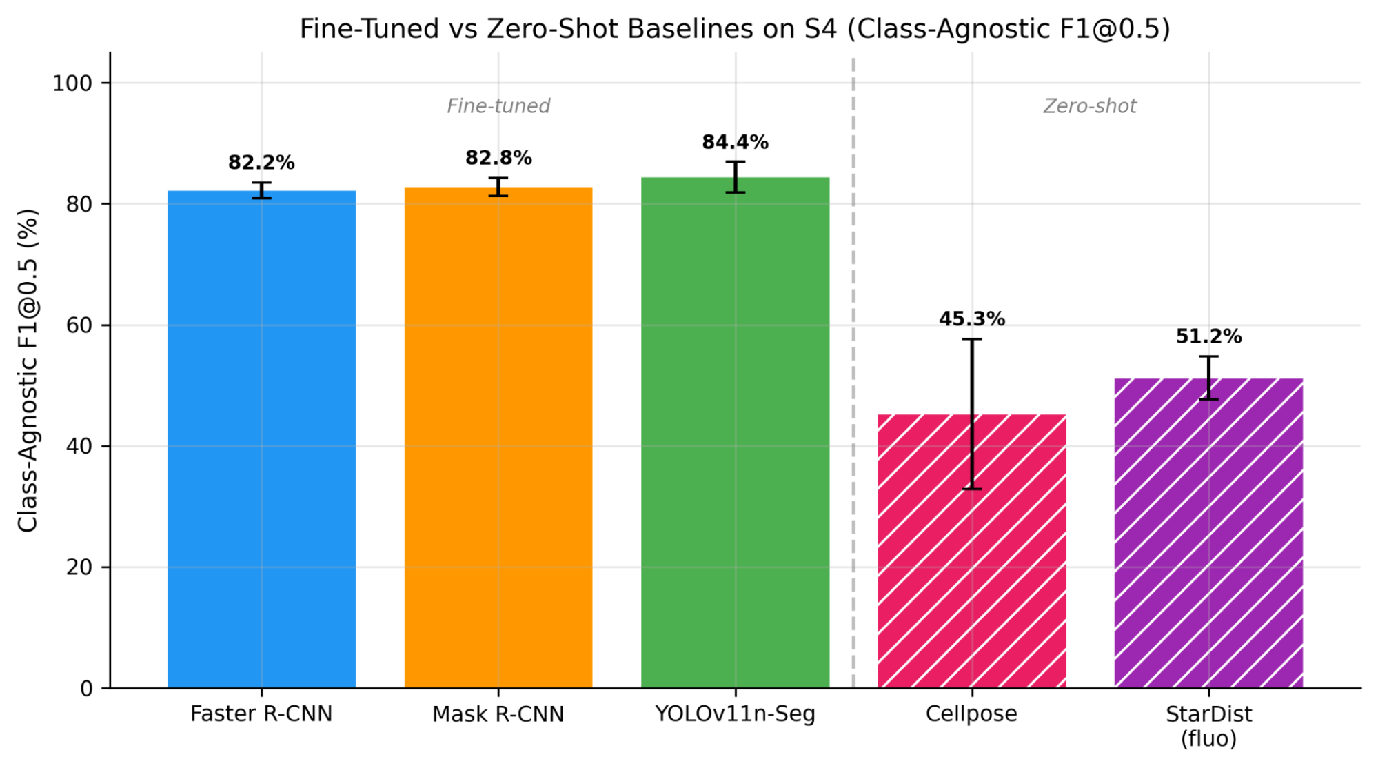
Figure 9. Fine-tuned models vs. zero-shot generalist baselines on S4. Using class-agnostic F1@0.5 for all models, the best fine-tuned model (YOLOv11n-Seg, 85.7%) exceeds the best generalist (StarDist, 51.2%) by 34.5 points

Figure 10. Class-agnostic F1@0.5 across all scenarios. Fine-tuned models jump from ~52% (S1/S2) to ~83-86% (S3/S4) with patchification, while zero-shot baselines remain flat (~45-51%) regardless of preprocessing

5. Model Efficiency

Table 8 compares the computational cost of the fine-tuned models in the best-performing scenario (NVIDIA A100 GPU). YOLOv11n-Seg required only 2.6M parameters and 4.4 ms per patch, compared with 41.5M parameters and 25.4 ms for Faster R-CNN, and 44.2M parameters and 27.9 ms for Mask R-CNN. As visualized in Figure 11, YOLOv11n-Seg occupies the most favorable point on the accuracy-speed trade-off curve, combining the highest mAP50 with the fastest inference. Figure 12 shows that this advantage remains at mAP50-95, confirming that the speed gain does not come at the expense of precise localization.

The ~100 ms per image reported below decomposes as follows: grid detection + perspective warping of 16 patches runs in 35.7 ± 3.8 ms on a single CPU thread (measured on Apple M1; the Hough transform is the dominant cost at 25.9 ms), and YOLOv11n-Seg inference of 16 patches takes 16 × 4.4 = 70.4 ms on an A100. CPU and GPU stages can be pipelined in deployment, making the per-image wall-clock time approach the larger of the two.

From a deployment perspective, this result is highly relevant. Because one haemocytometer image corresponds to 16 patches, the reported inference time implies that a full image can be processed in approximately 100 ms. This makes near-real-time viability-aware cell counting feasible in practical microscopy workflows. At the same time, the full-resolution experiments suggest an important nuance: if patchification cannot be applied, the two-stage detectors remain more robust than YOLOv11n-Seg. Thus, YOLOv11n-Seg is the preferred model for the intended pipeline, but Faster R-CNN or Mask R-CNN may still be useful fallback options in less controlled acquisition settings.

Table 8. Model Efficiency Comparison (S4)

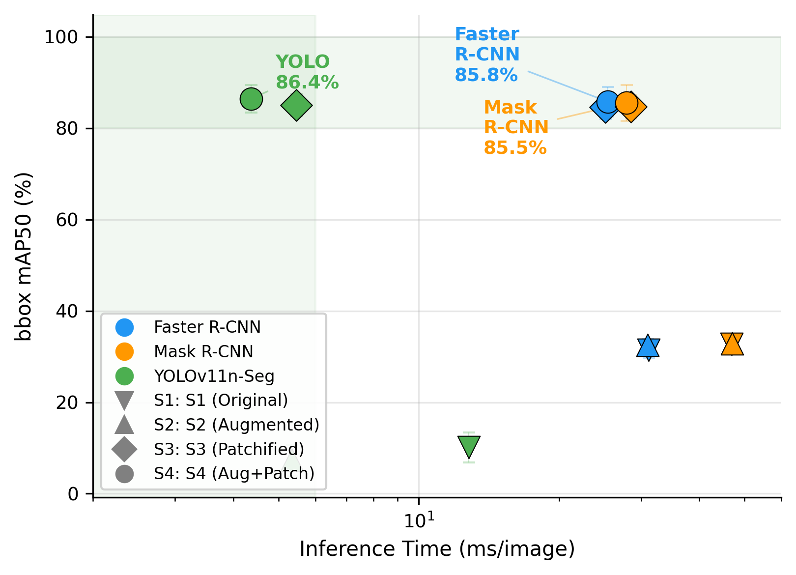
Figure 11. Accuracy (mAP50) vs. inference speed. YOLOv11n-Seg achieves the highest mAP50 (86.4%) at 6x faster inference than Faster R-CNN and Mask R-CNN, Pareto-dominating all alternatives

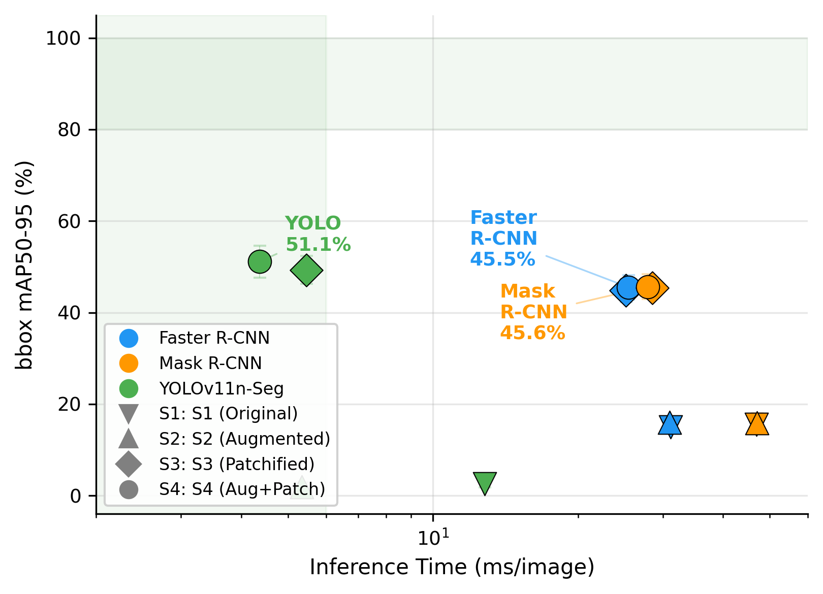
Figure 12. Accuracy (mAP50-95) vs. inference speed. YOLOv11n-Seg maintains its advantage at the stricter metric (51.1% vs. ~45% for Faster R-CNN and Mask R-CNN), indicating tighter bounding box localization

6. Comparison with Prior Work

Table 9 places our best bounding box mAP50 (86.4%) in context against three reference points from the literature. Against stained blood-cell detectors on the BCCD dataset [13],[15], our accuracy is ~7–9 points lower, an expected gap given the absence of chemical staining, the much smaller dataset (24 vs. 364+ images), and the morphological similarity of live and dead cells under brightfield. Against trypan-blue-stained cell counting [31] (F1 > 0.96), we are again lower, again attributable to the modality gap. The more informative comparison is against LIVECell [30], a large unstained brightfield benchmark of 1.6 M annotated cells: our segmentation mAP50-95 (~46%) sits within the performance band reported there despite our dataset being ~66,000× smaller, which we attribute to structure-aligned patchification compensating for the small-dataset disadvantage. The key takeaway is that staining variability (BCCD / trypan blue) and low contrast (LIVECell / our setting) pose different challenges. Patch-based tiling is the shared methodological insight across sub-literatures, but the structure-aligned variant we use here is tailored to the haemocytometer's native spatial units.

Table 9. Quantitative comparison with prior work (bounding box mAP50 and segmentation mAP50-95, %)

7. Practical Implications

Taken together, the results suggest several practical observations for laboratories considering automated cell segmentation or counting on haemocytometer images, with the caveat that all observations are drawn from this single dataset (24 images, RAW 264.7 macrophages, 100× unstained brightfield) and would benefit from external replication:

1. Preprocessing matters most. In our setting, grid-aligned patchification was the dominant factor for detection accuracy; without it, all three architectures we tested underperformed substantially. Whether this dominance generalizes to other haemocytometer protocols, magnifications, or cell types remains to be confirmed.
2. Full-resolution fallback. When patchification cannot be applied, two-stage detectors (Mask R-CNN in particular) were roughly 3× more robust than YOLOv11n-Seg on full-resolution images in our experiments.
3. Domain-specific training appears necessary in this modality. Zero-shot Cellpose and StarDist did not transfer adequately to unstained brightfield haemocytometer images in our deployment-mode comparison. Once patchification is applied, lightweight single-stage models become attractive for deployment. In this study, YOLOv11n-Seg offered the best overall balance of accuracy, localization, and runtime efficiency.
4. Throughput. With our preprocessing and model setup, a full 4×4 haemocytometer image was processed in approximately 100 ms (including grid detection), suggesting that real-time operation during microscopy sessions is plausible.

5. CONCLUSIONS

This study benchmarked five cell-detection approaches for automated macrophage viability assessment in unstained brightfield haemocytometer images under a controlled 2×2 factorial design. Grid-aligned patchification was identified as the single most impactful preprocessing step, improving mAP50 by 2.6–8.4× across all three fine-tuned architectures (paired Wilcoxon p = 0.016, Cohen's d > 3). A 2×2 ANOVA on per-fold bounding box mAP50 attributes 99.2–99.4% of explained variance to the patchification factor, with the augmentation main effect and the patchification × augmentation interaction each below 0.1%. On patched scenarios (S3, S4) the three fine-tuned models converge to 85.5–86.4% mAP50. YOLOv11n-Seg additionally dominates at the stricter mAP50-95 threshold (51.1% versus 45.5–45.6% for the two-stage models, a 5–6 point lead at a tighter localization criterion). Instance segmentation mAP50 tracks bounding-box mAP50 within 1–2 points on S4, so the detection-level gains carry over directly to shape recovery. A consistent per-class detection gap separates living (~93–95%) from dead (~78%) cells on S4 across all three architectures (14.4, 15.4, and 16.4 points for Faster R-CNN, Mask R-CNN, and YOLOv11n-Seg respectively) and the gap is statistically significant within each fold (paired one-sided Wilcoxon p = 0.0156, Cohen's d ≥ 3.5). The gap is morphology-driven and partly class-imbalance-driven. Under a unified class-agnostic F1@0.5 metric, fine-tuned models (82.2–84.4%) exceed the best zero-shot generalist (StarDist, 51.2%) by 31–33 percentage points, a lower bound on the gap under class-aware evaluation.

The best fine-tuned model (YOLOv11n-Seg, 86.4% mAP50, 51.1% mAP50-95, 4.4 ms per patch, 2.6 M parameters) processes a full 16-patch haemocytometer image in ~100 ms end-to-end (35.7 ms for grid detection on CPU and 70.4 ms for the 16 patch inferences on an A100 GPU), enabling near-real-time viability assessment during microscopy sessions and making edge deployment (smaller GPUs, laptop-class accelerators) plausible given the 17× smaller parameter count. Relative to published estimates for manual haemocytometer counting (~5–10 min per image), the automated pipeline represents a practical throughput gain of more than three orders of magnitude, with the additional benefit of removing operator fatigue and inter-observer variability. Theoretically, the variance decomposition reframes the prevailing intuition that augmentation and model choice drive biomedical small-object detection: for small, unstained, structure-aligned targets, a preprocessing step that respects the imaging protocol's native spatial units dominates both factors by two orders of magnitude.

The findings are derived from a single laboratory, a single cell line (RAW 264.7 macrophages), a single acquisition protocol (100× unstained brightfield), and a dataset of only 24 images (6,307 polygon annotations). Generalization to other cell types, staining conditions, magnifications, or haemocytometer brands has not been demonstrated and is the central open question. Dead-cell annotation relied on morphological cues alone rather than a chemical gold standard (e.g., trypan blue exclusion), so the per-class gap may overstate the "true" biological separability. A second annotator reviewed every image for the QC pass, but a formal inter-rater reliability study was not performed. The zero-shot generalist comparison is deliberately a deployment-mode evaluation. Fine-tuning Cellpose or StarDist on brightfield haemocytometer data is an obvious extension that would isolate architecture-level differences from deployment-mode ones. Patch size was fixed at 256×256 and not swept. In priority order, future work should therefore (1) address the per-class gap with class-weighted or focal loss and hard-example mining; (2) externally validate on public brightfield datasets and across labs; (3) sweep patch sizes and evaluate grid-detection robustness on other haemocytometer brands and illumination conditions; (4) fine-tune Cellpose and StarDist for a matched architectural comparison; (5) explore semi-supervised annotation to reduce the labeling burden; and (6) integrate the pipeline with robotic microscopy for fully automated viability assessment. We hope these results contribute to the broader adoption of deep learning in routine laboratory assays and provide a concrete, reproducible baseline for unstained brightfield haemocytometer analysis.

DECLARATION

Supplementary Materials

The dataset and code is available upon request. Please contact the corresponding author via email at mohammad.ikhsan04@ui.ac.id.

Sustainable Development Goals

This research contributes to SDG 3 (Good Health and Well-Being) by developing automated tools for cell viability assessment that can improve the efficiency and reproducibility of biomedical research in regenerative medicine, pharmacology, and cell biology.

Author Contribution

Mohammad Ikhsan: Conceptualization, Methodology, Software, Formal Analysis, Writing - Original Draft, Writing - Review & Editing. Zino Ramdani Suharto: Dataset - Curation, Investigation, Validation. Rizal Azis: Dataset - Collection & Annotation, Writing - Review & Editing. Basari: Resources, Writing - Review & Editing.

Funding

This research received no external funding.

Acknowledgement

The authors thank the Department of Electrical Engineering, Universitas Indonesia, for providing research support. Training was performed on Google Colab Pro with NVIDIA A100 GPUs.

Conflicts of Interest

The authors declare no conflict of interest.

Ethics and Data Provenance

The study used the RAW 264.7 macrophage cell line (commercially available as ATCC TIB-71); no human subjects, human tissue, or animal procedures were involved. Cell-line provenance was confirmed against the vendor specification prior to imaging. No personally identifiable information appears in the dataset, and no review by an ethics board was required.

ABBREVIATIONS

The following abbreviations are used in this manuscript.

REFERENCES

1. T. L. Riss, R. A. Moravec, A. L. Niles, S. Duellman, H. A. Benink, T. J. Worzella, and L. Minor, “Cell viability assays,” Assay guidance manual [Internet], 2016, https://www.ncbi.nlm.nih.gov/books/NBK574243/?report=reader.  
2. K. A. Patel et al., “Validation of Automated Fluorescent-Based Technology for Measuring Total Nucleated Cell Viability of Hematopoietic Progenitor Cell Products,” Transfusion (Paris), vol. 62, no. 4, pp. 848–856, 2022, https://doi.org/10.1111/trf.16837.
3. W. Strober, “Trypan Blue Exclusion Test of Cell Viability,” Curr. Protoc. Immunol., vol. 111, no. 1, p. A3.B.1-A3.B.3, 2015, https://doi.org/10.1002/0471142735.ima03bs111.
4. Y. Chen and P.-J. Chiang, “An Automated Approach for Hemocytometer Cell Counting Based on Image-Processing Method,” Measurement, vol. 234, p. 114894, 2024, https://doi.org/10.1016/j.measurement.2024.114894.
5. K. Hildebrand et al., “AI-Driven Analysis for Real-Time Detection of Unstained Microscopic Cell Culture Images,” AI, vol. 6, no. 10, p. 271, 2025, https://doi.org/10.3390/ai6100271.

6. Z. Zou, K. Chen, Z. Shi, Y. Guo, and J. Ye, “Object Detection in 20 Years: A Survey,” Proc. IEEE, vol. 111, no. 3, pp. 257–332, 2023, https://doi.org/10.1109/jproc.2023.3238524.
7. R. Morelli et al., “Automating Cell Counting in Fluorescent Microscopy through Deep Learning with c-ResUnet,” Sci. Rep., vol. 11, no. 1, 2021, https://doi.org/10.1038/s41598-021-01929-5.
8. Y. Liu et al., “Cell Counting in the Era of Deep Learning: Methods and Challenges,” Cell Transplant., vol. 33, 2024, https://doi.org/10.1177/09636897241293628.
9. J. Ma et al., “The Multimodality Cell Segmentation Challenge: Toward Universal Solutions,” Nat. Methods, vol. 21, no. 6, pp. 1103–1113, 2024, https://doi.org/10.1038/s41592-024-02233-6.
10. S. Ren, K. He, R. Girshick and J. Sun, "Faster R-CNN: Towards Real-Time Object Detection with Region Proposal Networks," in IEEE Transactions on Pattern Analysis and Machine Intelligence, vol. 39, no. 6, pp. 1137-1149, 2017, https://doi.org/10.1109/TPAMI.2016.2577031.  

11. J. Redmon, S. Divvala, R. Girshick, and A. Farhadi, “You Only Look Once: Unified, Real-Time Object Detection,” in Proceedings of the IEEE Conference on Computer Vision and Pattern Recognition, pp. 779–788, 2016, https://doi.org/10.1109/cvpr.2016.91.
12. J. Terven, D.-M. Cordova-Esparza, and J.-A. Romero-Gonzalez, “A Comprehensive Review of YOLO Architectures in Computer Vision: From YOLOv1 to YOLOv8 and YOLO-NAS,” Mach. Vis. Appl., vol. 34, no. 6, p. 116, 2023, https://doi.org/10.1007/s00138-023-01426-z.
13. P. Mehta et al., “Benchmarking YOLO Variants for Enhanced Blood Cell Detection,” Int. J. Imaging Syst. Technol., vol. 35, no. 1, 2025, https://doi.org/10.1002/ima.70037.
14. Y. He, “Automatic Blood Cell Detection Based on Advanced YOLOv5s Network,” IEEE Access, vol. 12, pp. 17639–17650, 2024, https://doi.org/10.1109/access.2024.3360142.
15. X. Chen et al., “NBCDC-YOLOv8: A new framework to improve blood cell detection and classification based on YOLOv8,” IET Comput. Vis., vol. 19, no. 1, 2025, https://doi.org/10.1049/cvi2.12341.

16. D. Zhang et al., “TW-YOLO: An Innovative Blood Cell Detection Model Based on Multi-Scale Feature Fusion,” Sensors, vol. 24, no. 19, p. 6168, 2024, https://doi.org/10.3390/s24196168.
17. M. G. Ragab et al., “A Comprehensive Systematic Review of YOLO for Medical Object Detection (2018 to 2023),” IEEE Access, vol. 12, pp. 57815–57836, 2024, https://doi.org/10.1109/access.2024.3386826.
18. H. Sazak and M. Kotan, “Automated Blood Cell Detection and Classification in Microscopic Images Using YOLOv11 and Optimized Weights,” Diagnostics, vol. 15, no. 1, p. 22, 2024, https://doi.org/10.3390/diagnostics15010022.
19. K. He, G. Gkioxari, P. Dollár, and R. Girshick, “Mask R-CNN,” in Proceedings of the IEEE International Conference on Computer Vision, pp. 2961–2969, 2017, https://doi.org/10.1109/ICCV.2017.322.  
20. M. Hu et al., “An Improved Mask R-CNN Model for Cell Detection and Segmentation in Microscopy Images,” Sensors, vol. 24, no. 8, p. 2424, 2024, https://doi.org/10.3390/s24082424.

21. G. Moallem et al., “Detecting and Counting Unstained and Unmanipulated Adherent Cells in Brightfield by Faster Region-Based Convolutional Neural Network,” J. Biomed. Opt., vol. 27, no. 7, p. 076003, 2022, https://doi.org/10.1117/1.jbo.27.7.076003.
22. T.-Y. Lin et al., “Microsoft COCO: Common Objects in Context,” in European Conference on Computer Vision, pp. 740–755, 2014, https://doi.org/10.1007/978-3-319-10602-1_48.
23. K. He, X. Zhang, S. Ren, and J. Sun, “Deep Residual Learning for Image Recognition,” in Proceedings of the IEEE Conference on Computer Vision and Pattern Recognition, pp. 770–778, 2016,https://doi.org/10.1109/cvpr.2016.90.  
24. G. Zhan et al., “Auto-CSC: A Transfer Learning Based Automatic Cell Segmentation and Count Framework,” Cyborg Bionic Syst., vol. 2022, p. 9842349, 2022, https://doi.org/10.34133/2022/9842349.
25. X. Wang et al., “Induced Pluripotent Stem Cells Detection via Ensemble YOLO Network,” in Proceedings of the Annual International Conference of the IEEE Engineering in Medicine and Biology Society, pp. 3738–3741, 2021, https://doi.org/10.1109/embc46164.2021.9629744.

26. C. Xu et al., “Transfer Learning and SE-ResNet152 Networks-Based for Small-Scale Unbalanced Cervical Cell Detection,” Diagnostics, vol. 12, no. 10, p. 2477, 2022, https://doi.org/10.3390/diagnostics12102477.  
27. C. Stringer, T. Wang, M. Michaelos, and M. Pachitariu, “Cellpose: a generalist algorithm for cellular segmentation,” Nat. Methods, vol. 18, no. 1, pp. 100–106, 2021, https://doi.org/10.1038/s41592-020-01018-x.
28. M. Pachitariu and C. Stringer, “Cellpose 2.0: how to train your own model,” Nat. Methods, vol. 19, no. 12, pp. 1634–1641, 2022, https://doi.org/10.1038/s41592-022-01663-4.
29. U. Schmidt, M. Weigert, C. Broaddus, and G. Myers, “Cell Detection with Star-Convex Polygons,” in Medical Image Computing and Computer Assisted Intervention – MICCAI 2018, pp. 265–273, 2018, https://doi.org/10.1007/978-3-030-00934-2_30.
30. C. Edlund et al., “LIVECell—A large-scale dataset for label-free live cell segmentation,” Nat. Methods, vol. 18, no. 9, pp. 1038–1045, 2021, https://doi.org/10.1038/s41592-021-01249-6.

31. L. Kuijpers et al., “Automated cell counting for Trypan blue-stained cell cultures using machine learning,” PLOS ONE, vol. 18, no. 11, p. e0291625, 2023, https://doi.org/10.1371/journal.pone.0291625.
32. K. Hoyos and W. Hoyos, “Supporting Malaria Diagnosis Using Deep Learning and Data Augmentation,” Diagnostics, vol. 14, no. 7, p. 690, 2024, https://doi.org/10.3390/diagnostics14070690.
33. D. Fishman et al., “Practical Segmentation of Nuclei in Brightfield Cell Images with Neural Networks Trained on Fluorescently Labelled Samples,” J. Microsc., vol. 284, no. 1, pp. 12–24, 2021, https://doi.org/10.1111/jmi.13038.
34. M. A. S. Ali et al., “Evaluating Very Deep Convolutional Neural Networks for Nucleus Segmentation from Brightfield Cell Microscopy Images,” SLAS Discov., vol. 26, no. 9, pp. 1125–1137, 2021, https://doi.org/10.1177/24725552211023214.
35. M. Vašinková et al., “Comparing Deep Learning Performance for Chronic Lymphocytic Leukaemia Cell Segmentation in Brightfield Microscopy Images,” Bioinforma. Biol. Insights, vol. 18, 2024, https://doi.org/10.1177/11779322241272387.

36. S. Korkut, C. Erkan, and S. Aksoy, “On the benefits of region of interest detection for whole slide image classification,” in Proceedings of SPIE, 2023. https://doi.org/10.1117/12.2654193.
37. D. K. Ufuktepe et al., “Cell Patch Extraction for Malaria Detection Using Deep Learning,” in IEEE Applied Imagery Pattern Recognition Workshop, 2021. https://doi.org/10.1109/aipr52630.2021.9762109.
38. F. C. Akyon, S. O. Altinuc, and A. Temizel, “Slicing Aided Hyper Inference and Fine-Tuning for Small Object Detection,” in IEEE International Conference on Image Processing, pp. 966–970, 2022,https://doi.org/10.1109/icip46576.2022.9897990.
39. F. O. Unel, B. O. Ozkalayci, and C. Cigla, “The Power of Tiling for Small Object Detection,” in 2019 IEEE/CVF Conference on Computer Vision and Pattern Recognition Workshops (CVPRW), Long Beach, CA, USA: IEEE, Jun. pp. 582–591, 2019, https://doi.org/10.1109/CVPRW.2019.00084.
40. S. Das, G. Roy, and P. Zun, “High-Throughput Low-Cost Segmentation of Brightfield Microscopy Live Cell Images,” arXiv preprint arXiv:2508.14106, 2025, https://doi.org/10.48550/arXiv.2508.14106.  

41. G. Moallem, A. A. Pore, A. Gangadhar, H. Sari-Sarraf, and S. A. Vanapalli, “Detection of live breast cancer cells in bright-field microscopy images containing white blood cells by image analysis and deep learning,” J. Biomed. Opt., vol. 27, no. 07, 2022, https://doi.org/10.1117/1.JBO.27.7.076003.
42. H. Li et al., “Machine-Learning-Assisted Automatic Counting of Fungal Cells in a Hemocytometer,” Eng. Life Sci., vol. 21, no. 12, pp. 835–844, 2021, https://doi.org/10.1002/elsc.202100055.
43. S. Nakarmi et al., “Deep-Learning Assisted Detection and Quantification of (oo)Cysts of Giardia and Cryptosporidium on Smartphone Microscopy Images,” J. Mach. Learn. Biomed. Imaging, vol. 2, pp. 956–976, 2024, https://doi.org/10.59275/j.melba.2024-a333.
44. A. Kirillov et al., Segment anything. In Proceedings of the IEEE/CVF international conference on computer vision, pp. 4015-4026, 2023, https://doi.org/10.1109/ICCV51070.2023.00371.  
45. A. Kos, D. Belter, and K. Majek, “Deep Learning for Small and Tiny Object Detection: A Survey,” Pomiary Autom. Robot., vol. 27, no. 3, pp. 85–94, 2023, https://doi.org/10.14313/par_249/85.

46. F. A. Shewajo and K. A. Fante, “Tile-based microscopic image processing for malaria screening using a deep learning approach,” BMC Med. Imaging, vol. 23, no. 1, p. 39, 2023, https://doi.org/10.1186/s12880-023-00993-9.
47. F. Abdurahman, K. A. Fante, and M. Aliy, “Malaria parasite detection in thick blood smear microscopic images using modified YOLOV3 and YOLOV4 models,” BMC Bioinformatics, vol. 22, no. 1, p. 112, 2021, https://doi.org/10.1186/s12859-021-04036-4.
48. T.-Y. Lin, P. Dollár, R. Girshick, K. He, B. Hariharan, and S. Belongie, “Feature Pyramid Networks for Object Detection,” in Proceedings of the IEEE Conference on Computer Vision and Pattern Recognition, pp. 2117–2125, 2017, https://doi.org/10.1109/cvpr.2017.106.
49. N. E. M. Khalifa, M. Loey, and S. Mirjalili, “A Comprehensive Survey of Recent Trends in Deep Learning for Digital Images Augmentation,” Artif. Intell. Rev., vol. 55, no. 3, pp. 2351–2377, 2022, https://doi.org/10.1007/s10462-021-10066-4.
50. P. Chlap et al., “A Review of Medical Image Data Augmentation Techniques for Deep Learning Applications,” J. Med. Imaging Radiat. Oncol., vol. 65, no. 5, pp. 545–563, 2021, https://doi.org/10.1111/1754-9485.13261.

51. A. Kebaili, J. Lapuyade-Lahorgue, and S. Ruan, “Deep Learning Approaches for Data Augmentation in Medical Imaging: A Review,” J. Imaging, vol. 9, no. 4, p. 81, 2023, https://doi.org/10.3390/jimaging9040081.
52. R. Sapkota and M. Karkee, “Ultralytics YOLO evolution: An overview of YOLO26, YOLO11, YOLOv8 and YOLOv5 object detectors for computer vision and pattern recognition,” arXiv preprint arXiv:2510.09653, 2025, https://doi.org/10.48550/arXiv.2510.09653.
53. R. Khanam and M. Hussain, “YOLOv11: An Overview of the Key Architectural Enhancements,” arXiv:2410.17725, 2024, https://doi.org/10.48550/arXiv.2410.17725.