ISSN: 2685-9572 Buletin Ilmiah Sarjana Teknik Elektro
Vol. 8, No. 2, April 2026, pp. 395-407
Improving Mobile Robot Navigation Using Deep Q-Learning with Diagonal Motion under Dynamic Obstacle Environments
Karam A. Al-Zubaidi, Ahmed M. Alkamachi, Bahaa Ansaf
Department of Mechatronics Engineering, Al-Khawarizmi College of Engineering, University of Baghdad, Baghdad, Iraq
ARTICLE INFORMATION |
| ABSTRACT |
Article History: Received 17 December 2025 Revised 03 March 2026 Accepted 03 April 2026 |
| 
Navigation of the mobile robot in dynamic environments is a significant challenge for researchers due to the uncertainty and rapid changes in obstacle movement. This study proposes a framework for navigating a mobile robot using a deep Q-learning (DQL) algorithm in environments containing both static and dynamic obstacles. The research contribution lies in integrating diagonal motion to enhance manoeuvrability and improve decision-making under dynamic conditions. This paper compares the model with the basic motions model (front, back, right, left). The comparison is conducted across four environments of varying difficulty in terms of the density of obstacles. The model is trained by 3000 episodes using a Deep Q-Network (DQN) with two fully connected hidden layers consisting of 128 and 64 neurons, respectively, employing a greedy policy and utilizes a LiDAR simulator for spatial perception. Both models achieved a 100% success rate in reaching the target without collision in environments A and B, and 90% in environments C and D. However, the proposed approach succeeded in reducing the average number of steps required to reach the goal in all four environments, shortening the path by 10% to 20%. This reduces the time and energy required to reach the goal, which is a significant and crucial advantage in real-world environments. Even when tested at obstacle speeds up to six times the robot's speed, it demonstrated superiority compared to the other model. The model showed very good performance even with noise on the LiDAR reading. In short, the proposed model offers a robust and scalable approach to mobile robot navigation in real-world environments. |
Keywords: Dynamic Obstacle; Grid Environment; Deep Q-Learning; Mobile Robot Navigation; Discrete Action Space |
Corresponding Author: Ahmed M. Alkamachi, Department of Mechatronics Engineering, Al-Khawarizmi College of Engineering, University of Baghdad, Baghdad, Iraq. Email: ahmed78@kecbu.uobaghdad.edu.iq |
This work is open access under a Creative Commons Attribution-Share Alike 4.0 
|
Document Citation: K. A. Al-Zubaidi, A. M. Alkamachi, and B. Ansaf, “Improving Mobile Robot Navigation Using Deep Q-Learning with Diagonal Motion under Dynamic Obstacle Environments,” Buletin Ilmiah Sarjana Teknik Elektro, vol. 8, no. 2, pp. 395-407, 2026, DOI: 10.12928/biste.v8i2.15637. |
- INTRODUCTION
Even with processing technology advancements, Mobile robots continue to attract the interest of researchers and are becoming increasingly economically viable [1]-[3]. Navigating crowded spaces is crucial for practical applications such as warehouse automation and service robots, as well as self-driving cars and mobile robots [4]-[6].
In an age characterized by artificial intelligence, it has become essential to develop intelligent algorithms for planning robot routes [7]-[9]. However, the latter is resource-intensive on perception, planning and control systems for a variety of reasons, such as partial observability of the environment; unpredictability in motion of dynamic obstacles; computational constraints that real-time processors experience; vehicle dynamics preservation and generation of collision-free trajectories [10]-[12].
Several studies have addressed the guidance of mobile robots to avoid obstacles. In [13]-[15], these studies suggested a Dynamic Window Approach (DWA) algorithm for robot path planning. In another study, the D* algorithm is used to determine the path of the mobile robot [16]. Many studies have used prominent algorithms in path planning, such as the Timed-Elastic-Bands (TEB), EBS-A*, A* algorithm, Probabilistic Roadmap (PRM) [17]-[21].
When it comes to avoiding moving obstacles, deep reinforcement learning systems outperformed traditional algorithms [22][23]. Research into deep reinforcement learning algorithms used for dynamic obstacle avoidance in mobile robots has arisen as a crucial topic of investigation due to the rising demand for autonomous navigation in complex and unexpected situations [24][25].
Modern research in RL-based mobile robot navigation ranges from various algorithms and architectural improvements, considering the peculiarities of moving obstacle avoidance. The performance of the RL algorithm is determined to a large extent and varies among methods in dependence on sensor modality, environmental complexity, and task requirements [26]. This includes the Deep Q-Networks (DQN), Double DQN, and Proximal Policy Optimization (PPO) algorithms, resulting in more effective, flexible, and scalable systems [27]-[32]. Deep neural networks are capable of developing efficient control methods using sensor inputs, allowing them to adapt to changes in the environment without the need for retraining [33][34].
With such advances, the challenge of avoiding moving obstacles is still faced by robots when they cannot predict the obstacle motion and get limitations on sensor information as well as limited generalization to real situations [35]-[37]. Research revealed a knowledge gap of theoretical studies in developing algorithms capable of optimize both navigation performance and safety for real-life cases [38]-[42]. In addition, the best reinforcement learning algorithms and reward function design is an ongoing debate. Some advocate value-based methods, such as DQN, and others choose policy gradient methods for continuous control, like DDPG, SAC and TD3 [43]-[48]. Such knowledge gaps have several consequences that are related to the poorer navigational performance, heightened crash risk and problems associated with transitioning designs to realistic application [49][50].
The key academic contribution of this work is the solution to the robot Navigation problem in an environment with both static and dynamic obstacles using a Deep Q-Learning (DQL) within a guiding framework for a 15x15 grid environment, where obstacles move randomly, achieving improved navigation efficiency and a 10–20% reduction in path length through the use of diagonal motion actions The proposed method utilizes the custom reward function to promote fast convergence and avoid collisions and slow behaviors, whose effectiveness is tested in different obstacle speeds. The method for the mobile robot can move diagonally, so the agent can go in more directions to avoid moving obstacles and take a shorter path. In the course of our optimal Navigation decision process, the agent is able to sense its surroundings through simulated LiDAR sensing. Evaluate the model under different noise on the LiDAR reading. The research paper includes a comparison with the DQL algorithm for an agent that moves in the four basic steps to show the difference made by diagonal movement. The effectiveness of the proposed approach is evaluated using standard navigation performance metrics, including success rate and path efficiency.
In this study, the Deep Learning Q (DQL) algorithm is used as it is considered a fundamental standard in the field of reinforcement learning research. Although more advanced algorithmsو such as Proximal Policy Optimization (PPO), Soft Actor-Critic (SAC), could be used, DQL provides a more interpretable and clearer basis for studying the effects of diagonal motion and environmental dynamics, making it a useful basic reference that can later be developed into more advanced algorithms.
- METHODS
This section describes the training process of a mobile robot operating with the DQL algorithm to avoid static and moving obstacles in a 15×15 grid environment. A simulated LiDAR sensor is used to perceive its surroundings. A custom reward function is designed to encourage the robot to avoid obstacles and reach the goal in the fewest possible steps. An ε-greedy policy is employed to balance exploration and exploitation.
- Environment Setup
The agent is trained in a 15×15 grid environment containing randomly moving obstacles that are randomly repositioned in each episode. The robot's initial position is at (0,0) and the goal position is at (14,14). Each training episode ended when one of three conditions is met: colliding with an obstacle, reaching the allowed number of steps (200 steps), or successfully reaching the goal without any collision.
- State Representation
The state (S) is a 10-dimensional vector defined as follows:
| 
| (1) |
Where ( ) is robot’s current state (pose), (
 ) is goal position, G is grid size,
  is normalized robot and goal position,
  is normalized LiDAR reading in direction i (front, back, right, left, diagonal right-up, diagonal left-up), where
  is the number of cells to the nearest obstacle, and R is the LIDAR range (3 cells).
- Action space
The robot has six discrete actions a∈{0,1,2,3,4,5} that map to the movement directions:
| 
| (2) |
Diagonal down actions are excluded to avoid backward motion and maintain goal-directed navigation efficiency.
- Reward Function and Euclidean Distance
- Reward Function
As opposed to a typical reward function, which rewards a robot only when it arrives at the goal, this reward function is designed to encourage the agent to reach the goal in the shortest possible steps and to reduce wasteful movements by penalizing actions that take the agent further from the goal and rewarding actions that bring them closer. There is also a strict penalty for collisions, making the agent more efficient at avoiding obstacles and reaching the goal. The function of the reward is explained as follows:
| 
| (3) |
- Euclidean Distance
To establish if the robot has moved closer or further from the goal, the Euclidean distance between the Robot’s instantaneous position and the goal is calculated before and after the movement:
| 
| (4) |
- Distance Difference
The reward value is evaluated based on the change in distance ( ):
):
| 
| (5) |
Where  is the distance to the goal prior to taking action,
  is the distance from the goal after taking action. Interpretation: If > 0 is The robot is Approaching → +0.2, If < 0 is The robot is distancing. → -0.2, and If = 0 is No improvement → -0.1.
- Q-Network Architecture
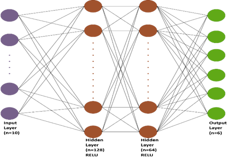
Used a deep Q-Network (DQN) with two hidden layers (128-64), fully connected, which allows the model to learn complex patterns. The Deep Q-Network (DQN) used has the following structure in Figure 1.
Figure 1. Structural design of the neural network
- Training Procedure
Training is done over N=3000 episodes, The agent uses the ε-greedy policy to choose an action at each stage. Begin with ε= 0.99 and gradually decrease by 0.995 every episode until it reaches 0.01.
| 
| (6) |
At each step, the agent chooses an action using:
| 
| (7) |
Where  is the evaluated Q-value for doing action a in state s, and denotes the expected cumulative future reward, Ѳ is refers to the trainable Variables (weights and biases) of the Q-network. Transitions are preserved in a replay memory. To update the Q-values, a mini-batch is sampled using the Bellman equation:
| 
| (8) |
Where  is the immediate reward received while performing action
  in state
  ,
,  is the discount factor (0.95) determines the relevance of future rewards,
  is the next state reached after doing action a,
  is all conceivable actions for the following state ,
  is the highest anticipated Q-value for the following state among all feasible actions, "terminal state" is denotes a condition in which the episode terminates, such as achieving the goal or colliding with an obstacle. The Q-network is updated by reducing the mean squared error between the goal value and the current forecast, using the following loss function:
| 
| (9) |
In Figure 2 depicts the DQL algorithm's sequence of operations.
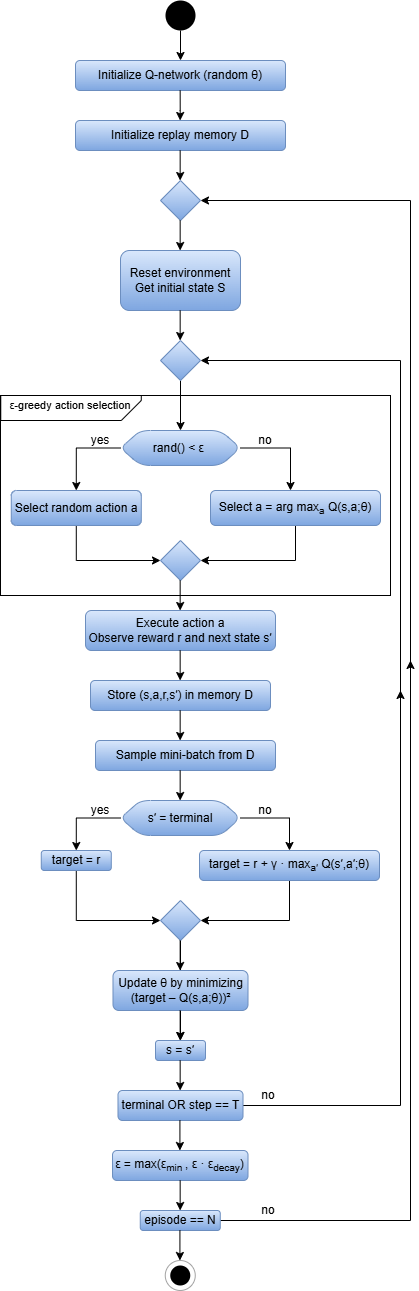
Figure 2. Structure of the Deep Q-Learning framework
- Computational Settings
The training parameters are carefully selected to ensure consistent convergence during the learning process. The replay memory is set up to hold 2000 experiences, with a minibatch size of 32 drawn at each update episode. The Adam optimizer is utilized to train the Q-network with a learning rate of 0.001 and an MSE loss function. The discount factor γ of 0.95 is used to weight present and future returns throughout training. The system is implemented with Python 3.12.7. Note that the neural network is implemented with the TensorFlow library, and the simulation environment is implemented with the use of the Matplotlib library. All computation is performed on a machine with an Intel i7 processor and 8GB RAM. All parameters, the reward function, and the size of the neural network, LiDAR range are chosen according to the specifications of the research paper [51], in order to ensure a fair comparison.
- RESULTS AND DISCUSSION
Analysis of the model’s training data will be shown in this section. Testing the model on varying difficulty in four environments, and comparing it to a model that works with non-diagonal motion to show the discrepancies. The contrast will be based on two primary measures: the amount of Success and the average number of steps to success. Furthermore, the section presents the images of environments and paths of each model.
- Training Analysis
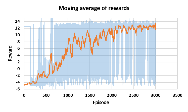
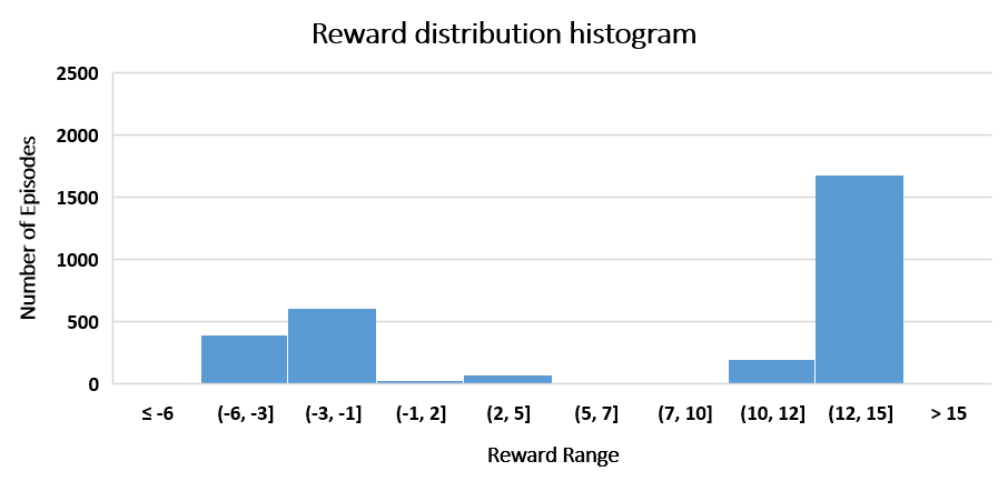
Data from 3000 training sessions are analyzed. Figure 3 shows the reward values during the training period. Figure 3(a) represents the moving average of the reward values, which started with negative values and gradually improved. Figure 3(b) shows the statistics of the reward values during the training.
|
[a] |
|
[b] |
Figure 3. Reward evaluation during training, [a] Moving average of rewards, [b] Reward distribution histogram
As illustrated in Figure 4, the increasing success rates during training are shown. Figure 4(a) and Figure 4(b) show that from episodes 200 to 300, the model achieved one success, while by the end of episodes 2900-3000, it had achieved 93 successes. Figure 4(c) represents the increasing success curve, while Figure 4(d) presents statistics on the number of successes and failures across 3000 training episodes, with green representing successes and red representing failures to achieve the goal.
Figure 4. Analysis of agent success across training episodes: [a] Successes during episodes 200-300, [b] Successes during episodes 2900-3000, [c] Success rate curve, [d] Success–Failure histogram
- Experimental Environments
Illustrates Figure 5, the environments used for testing. The 15×15 grid environments are designed to evaluate the two models and compare the performance of each model in each environment, where each environment contains fixed and moving obstacles with different distributions and numbers for each environment. The speed of the obstacle is equal to the speed of the robot. The difficulty of each environment varies, with increasing density of obstacles and narrow passages. The blue circle represents the robot, the red circles represent moving obstacles, the black squares represent stationary obstacles, and the green square represents the goal.
- Quantitative Comparison
A comparison is made between a model operating with a DQL algorithm that moves diagonally in addition to the four basic movements and a model operating with a DQL algorithm that just moves with the four basic movements (front, back, right, left). The comparison is made by testing each algorithm ten times in each of the four environments shown in Figure 5. The comparison is based on two criteria: the number of successes (success is defined as reaching the goal within 200 steps and without collision) and the rate of steps taken to reach the goal. The rate of steps is calculated by dividing the sum of the steps in the successful tests by the number of successful tests. The test results are shown in Table 1.
Figure 5. Testing environments
Table 1. Performance comparison between diagonal and non-diagonal DQL navigation
Environment | DQL with diagonal movement | DQL without diagonal movement |
Success rate | Average Steps | Success rate | Average Steps |
Environment A | 10/10 | 24.6 | 10/10 | 29.1 |
Environment B | 10/10 | 26.9 | 10/10 | 29.4 |
Environment C | 9/10 | 27.4 | 9/10 | 31.1 |
Environment D | 9/10 | 26.8 | 9/10 | 34.2 |
- Quantitative Analysis
The experimental findings presented in Table 1 compare the DQL algorithm with diagonal movement and another with only basic movements in four different difficulty environments. The results showed that both models have high success rates, indicating the algorithm's ability to create an efficient navigation path to reach the goal. However, the difference between the two models lies in the number of steps to reach the goal.
Both models got 10/10 in environments A and B. The steps-per-model difference is clear; it can be seen how a model that allows diagonal movements has achieved lower step-rates to achieve the goal. Move (24.6 and 26.9 steps) vs (29.1 and 29.4 steps). This is a consequence of the model's capability to minimize the literal length of a path, as its paths are more direct towards the goal, therefore not needing to perform as many turns and thus more efficient navigation occurs.
In both environments C and D, where the two models' performance showed success rates of 9/10, the obstacle density has an equivalent effect on their avoidance ability. But the diagonal motion was still more efficient, as with the diagonal model it took (27.4 and 26.8) steps while with the model using only basic motions it required (31.1 and 34.2) steps to reach the goal. This goes to show the contrast: having the capability of moving diagonally shapes up smooth paths, and the agent can maneuver with greater ease.
In general, the results demonstrates that diagonal motion tends to optimize pathfinding and stabilizes the tunings of the robot’s navigational behavior, particularly when encountering non-uniform obstacle distributions. While the performance is comparable between the two approaches, the number of steps difference increases by 10%∼20%, which implies that diagonal movement would be better in minimizing the steps regardless of the given environments. This further supports our claim that allowing diagonal moves is a useful extension for deep learning navigation algorithms, especially when they are used on physical robots, where how the energy and time it takes to reach the goal matter. Figure 6 illustrates the behavior of the algorithms in each environment. The blue path represents the DQL algorithm with diagonal movement, and the red path represents the DQL algorithm without diagonal movement.
Figure 6. Trajectories of DQL with and without Diagonal Motion Across Multiple Environments
- Performance Assessment Across Multiple Obstacle Velocities
The model is tested in a 15×15 grid environment under varying obstacle speeds. The results are shown in Table 2. The results in Table 2 illustrate the effect of obstacle speed on the performance of a DQL with diagonal motion and a DQL without diagonal motion. At speeds 1× and 2×, the performance of the two models is converging. At speed 1×, both models achieved a success rate of 10/10, while the model without diagonal motion dropped to 9/10 at speed 2×. The model with diagonal motion maintained a perfect success rate of 10/10.
As the speed increases to 3× and 4×, the difference becomes clear. The diagonal movement model keeps its performance roughly the same (10/10 at 3× and 9/10 at 4×), compared to a drop in performance of the non-diagonal movement model (7/10 at 3× and only 4/10 at 4×). This disparity corresponds to the fact that diagonal motion opens up quicker egress in which to escape moving obstacles before collision.
At higher speed (5× – 6×), the difference matters. The diagonal moving model consistently fares well regardless of the complicated environments (8/10 at 5× and 6×), while the other model falls apart (2/10 at 5× and completely crumbles to 0/10 at 6×). This indicates that when the navigation task is performed with a dynamic environment at high speeds, the model completely fails without the use of diagonal motion because it becomes drastically constrained in directionality and thus loses effectiveness in maneuverability.
Taken together, the results demonstrates that the inclusion of diagonal motion greatly increases the model's maneuverability and improves its reaction to sudden changes in obstacle positions. This emphasizes the critical nature of multidirectional motion in real robotics environments. Especially where collisions with high-speed, unpredictable dynamic obstacles are common. In addition, the fact that the model outperforms against most obstacle speeds confirms its higher versatility and efficiency compared to a non-diagonal motion model.
When obstacles move at high speeds, the environment changes more rapidly between successive observations, reducing the agent’s ability to react optimally within a discrete time step. These factors reflect real-world constraints such as limited reaction time and actuation delays, which inherently challenge autonomous navigation systems.
Table 2. Impact of obstacle speed on the success of the model
Obstacle Speed | DQL with Diagonal Motion | DQL without Diagonal Motion [51] |
1× mobile robot speed | 10/10 | 10/10 |
2× mobile robot speed | 10/10 | 9/10 |
3× mobile robot speed | 10/10 | 7/10 |
4× mobile robot speed | 9/10 | 4/10 |
5× mobile robot speed | 8/10 | 2/10 |
6× mobile robot speed | 8/10 | 0/10 |
- Robustness Evaluation under Various LiDAR Noise Levels
To evaluate the robustness of our proposed navigation algorithm, we experimented with the robot over a variety of LiDAR measurement noise conditions. To describe the model of noisy measurements is outlined as:
| 
| (10) |
| 
| (11) |
Where  Reading LiDAR after noise,
  random Gaussian noise,
  standard deviation of the noise.
Evaluated the navigation success rate over 10 trials for different noise levels. Where the speed of the obstacle is equal to the speed of the robot. The results are summarized in Table 3. The efficacy of the algorithm is perfectly robust against noisy levels (σ≤0.1), achieving 100% success rate. Up to a noise level of 0.2, the model still performed with an accuracy of 80%. But the success rate drastically decreases as noise increases beyond 0.2. Elevated sensor noise degrades the reliability of LiDAR measurements, leading to partial or inaccurate perception of obstacle positions. This factor reflects real-world constraints such as sensor uncertainty.
Table 3. Effect of LiDAR Measurement Noise on Navigation Success Rate
Noisy Measurement | Success |
0.0 | 10/10 |
± 0.05 | 10/10 |
± 0.1 | 10/10 |
± 0.2 | 8/10 |
± 0.3 | 3/10 |
± 0.4 | 2/10 |
± 0.5 | 0/10 |
- CONCLUSION AND FUTURE WORK
In this paper, a model of a mobile robot using the Deep Q-Learning (DQL) algorithm was introduced to optimizing path length and improving maneuverability both for stationary and moving obstacles. The academic contribution of this study is identified from the follow several points: (i) support the diagonal movement; (ii) design the equivalent function which can make robot reach goal, at the same time reduce redundant motion to minimum; (iii) evaluate the model under different speed of obstacle; (iv) evaluate the model under different noise on the LiDAR reading.
The results showed that the diagonal motion model outperformed the model that moved in four basic directions (forward, backward, right, left) without diagonal motion. Both models achieved the same success rates. The results also showed that the diagonal motion model required fewer steps to reach the goal, reducing the path by 10% to 20% in various environments. This reduces the time and energy required to reach the goal, which is a significant and crucial advantage in real-world settings.
However, when tested with multi-speed obstacles up to six times the robot's speed, the superiority of the model with diagonal motion became clearly evident, achieving a significantly 80% success rate at 6x speed versus 0%to the model without diagonal motion. The model showed very good performance even with noise on the LiDAR reading.
It should be noted that the current results are obtained in a simulated 2D environment, which may not fully capture all real-world uncertainties and dynamics. Future work will focus on implementing the approach on 3D platforms (such as Gazebo and ROS) to improve realism and create the model using complex algorithms like PPO or SAC to handle continuous action spaces, and conduct experiments on actual robots to assess their resilience under realistic settings.
REFERENCES
- K. Almazrouei, I. Kamel, and T. Rabie, “Dynamic Obstacle Avoidance and Path Planning through Reinforcement Learning,” Appl. Sci., vol. 13, no. 14, p. 8174, 2023, https://doi.org/10.3390/app13148174.
- K. Alnabulseih, A.-E.-R. Abd-EL-Rehim, M. B. Badawi, and R. Elgohary, “Enhancing Disaster Response Efforts with YOLOv8-based Human Detection in Mobile Robotics,” Int. Integr. Intell. Syst., vol. 2, no. 1, 2025, https://doi.org/10.21608/iiis.2025.292458.1036.
- G. Fragapane, H.-H. Hvolby, F. Sgarbossa, and J. O. Strandhagen, “Autonomous Mobile Robots in Hospital Logistics,” In IFIP international conference on advances in production management systems, pp. 672–679, 2020, https://doi.org/10.1007/978-3-030-57993-7_76.
- S. Liu, P. Chang, W. Liang, N. Chakraborty, and K. Driggs-Campbell, “Decentralized Structural-RNN for Robot Crowd Navigation with Deep Reinforcement Learning,” in 2021 IEEE international conference on robotics and automation (ICRA), pp. 3517–3524, 2021, https://doi.org/10.48550/arXiv.2011.04820.
- M. Caruso, E. Regolin, F. Julian, C. Verdù, S. A. Russo, and S. Seriani, “Robot Navigation in Crowded Environments: A Reinforcement Learning Approach,” Machines, vol. 11, no. 2, pp. 1–29, 2023, https://doi.org/10.20944/preprints202212.0233.v1.
- T. T. Thuong and V. T. Ha, “Experimental Research on Avoidance Obstacle Control for Mobile Robots Using Q-Learning (QL) and Deep Q-Learning (DQL) Algorithms in Dynamic Environments,” In Actuators, vol. 13, no. 1, p. 26, 2023, https://doi.org/10.20944/preprints202311.0418.v1.
- C. Wang, X. Yang, and H. Li, “Improved Q-Learning Applied to Dynamic Obstacle Avoidance and Path Planning,” IEEE Access, vol. 10, pp. 92879–92888, 2022, https://doi.org/10.1109/ACCESS.2022.3203072.
- R. Raj and A. Kos, “A Comprehensive Study of Mobile Robot: History, Developments, Applications, and Future Research Perspectives,” Appl. Sci., vol. 12, no. 14, p. 6951, Jul. 2022, https://doi.org/10.3390/app12146951.
- N. Demir, P. Demircioğlu, and İ. Böğrekci, “Advancing Industry 4.0 With Ros: A Case Study On Autonomous Mobile Robot Technological Advancements,” Int. J. 3D Print. Technol. Digit. Ind., vol. 8, no. 1, pp. 130–142, 2024, https://doi.org/10.46519/ij3dptdi.1366132.
- U. Patel, N. K. Sanjeev Kumar, A. J. Sathyamoorthy, and D. Manocha, “DWA-RL: Dynamically Feasible Deep Reinforcement Learning Policy for Robot Navigation among Mobile Obstacles,” Proc. - IEEE Int. Conf. Robot. Autom., vol. 2021-May, pp. 6057–6063, 2021, https://doi.org/10.1109/ICRA48506.2021.9561462.
- Y. F. Chen, M. Everett, M. Liu, and J. P. How, “Socially aware motion planning with deep reinforcement learning,” in 2017 IEEE/RSJ International Conference on Intelligent Robots and Systems (IROS), pp. 1343–1350, 2017, https://doi.org/10.48550/arXiv.1703.08862.
- T. A. Fahmy, O. M. Shehata, and S. A. Maged, “Trajectory Aware Deep Reinforcement Learning Navigation Using Multichannel Cost Maps,” Robotics, vol. 13, no. 11, p. 166, 2024, https://doi.org/10.3390/robotics13110166.
- Z. Zhang, Y. Xue, N. Figueroa and K. Åkesson, "Gradient Field-Based Dynamic Window Approach for Collision Avoidance in Complex Environments," 2025 IEEE/RSJ International Conference on Intelligent Robots and Systems (IROS), pp. 19669-19674, 2025, https://doi.org/10.1109/IROS60139.2025.11246091.
- H. Qin, S. Shao, T. Wang, Y. Li, N. Wang, and C. Yao, “An Improved Dynamic Window Approach for Mobile Robot Dynamic Path Planning,” in 2022 12th International Conference on CYBER Technology in Automation, Control, and Intelligent Systems (CYBER), pp. 348–353, 2022, https://doi.org/10.1109/CYBER55403.2022.9907305.
- J. Kong and J. Cheng, “Path Planning of Mobile Robots Based on the Fusion of an Improved A* Algorithm and a Dynamic Window Approach,” in 2023 IEEE 6th Information Technology,Networking,Electronic and Automation Control Conference (ITNEC), pp. 968–973, 2023, https://doi.org/10.1109/ITNEC56291.2023.10082080.
- J. Guo, L. Liu, Q. Liu, and Y. Qu, “An Improvement of D* Algorithm for Mobile Robot Path Planning in Partial Unknown Environment,” in 2009 Second International Conference on Intelligent Computation Technology and Automation, pp. 394–397, 2009, https://doi.org/10.1109/ICICTA.2009.561.
- C. Rösmann, F. Hoffmann and T. Bertram, "Timed-Elastic-Bands for time-optimal point-to-point nonlinear model predictive control," 2015 European Control Conference (ECC), pp. 3352-3357, 2015, https://doi.org/10.1109/ECC.2015.7331052.
- Z. Liu, Z. Chang, C. Qiao, H. Chen, and G. Zong, “Improved Bidirectional A* and Time-Elastic Band Algorithm Based Mobile Robot Path Planning,” in 2025 37th Chinese Control and Decision Conference (CCDC), pp. 1–6, 2025, https://doi.org/10.1109/CCDC65474.2025.11090416.
- H. Wang, S. Lou, J. Jing, Y. Wang, W. Liu, and T. Liu, “The EBS-A* algorithm: An improved A* algorithm for path planning,” PLoS One, vol. 17, no. 2, pp. 1–27, 2022, https://doi.org/10.1371/journal.pone.0263841.
- F. Wang, W. Sun, P. Yan, H. Wei, and H. Lu, “Research on Path Planning for Robots with Improved A* Algorithm under Bidirectional JPS Strategy,” Appl. Sci., vol. 14, no. 13, 2024, https://doi.org/10.3390/app14135622.
- L. Qiao, X. Luo, and Q. Luo, “An Optimized Probabilistic Roadmap Algorithm for Path Planning of Mobile Robots in Complex Environments with Narrow Channels,” Sensors, vol. 22, no. 22, p. 8983, 2022, https://doi.org/10.3390/s22228983.
- J. Choi, G. Lee, and C. Lee, “Reinforcement learning-based dynamic obstacle avoidance and integration of path planning,” Intell. Serv. Robot., vol. 14, no. 5, pp. 663–677, 2021, https://doi.org/10.1007/s11370-021-00387-2.
- M. Likhachev and D. Ferguson, “Planning Long Dynamically Feasible Maneuvers for Autonomous Vehicles,” Int. J. Rob. Res., vol. 28, no. 8, pp. 933–945, 2009, https://doi.org/10.1177/0278364909340445.
- Y. Xi, “Research on Autonomous Mobile Robot Navigation Technology Based on Deep Reinforcement Learning,” Highlights Sci. Eng. Technol., vol. 114, pp. 108–113, 2024, https://doi.org/10.54097/krgznc69.
- M.-F. R. Lee and S. H. Yusuf, “Mobile Robot Navigation Using Deep Reinforcement Learning,” Processes, vol. 10, no. 12, pp. 1–22, 2022, https://doi.org/10.3390/pr10122748.
- A. P. Kalidas, C. J. Joshua, A. Quadir, S. Basheer, S. Mohan, and S. Sakri, “Deep Reinforcement Learning for Vision-Based Navigation of UAVs in Avoiding Stationary and Mobile Obstacles,” vol. 7, no. 4, pp. 1–23, 2023, https://doi.org/10.3390/drones7040245.
- Z. Zhang, “Path Planning Algorithms for Mobile Robots Based on Deep Reinforcement Learning,” Highlights Sci. Eng. Technol., vol. 114, pp. 49–55, 2024, https://doi.org/10.54097/fa2r8310.
- M. El Wafi, M. A. Youssefi, R. Dakir, and M. Bakir, “Intelligent Robot in Unknown Environments : Walk Path Using Q-Learning and Deep Q-Learning,” Automation, vol. 6, no. 1, p. 12, 2025, https://doi.org/10.3390/automation6010012.
- K. Sivayazi and G. Mannayee, “Modeling and simulation of a double DQN algorithm for dynamic obstacle avoidance in autonomous vehicle navigation,” e-Prime - Adv. Electr. Eng. Electron. Energy, vol. 8, p. 100581, 2024, https://doi.org/10.1016/j.prime.2024.100581.
- R. A, “Deep Reinforcement Learning with PPO for Autonomous Mobile Robot Navigation Using ROS 2 Framework,” Int. J. Res. Appl. Sci. Eng. Technol., vol. 13, no. 7, pp. 2119–2125, 2025, https://doi.org/10.22214/ijraset.2025.73330.
- S. M. Bankar and R. S. Pol, “Review on Optimizing Robotic Navigation with Deep Reinforcement Learning Algorithms,” J. Inf. Syst. Eng. Manag., vol. 10, no. 23s, pp. 226–237, 2025, https://doi.org/10.52783/jisem.v10i23s.3698.
- W. Zhu, X. Gao, H. Wu, J. Chen, X. Zhou, and Z. Zhou, “Design of Multimodal Obstacle Avoidance Algorithm Based on Deep Reinforcement Learning,” Electronics, vol. 14, no. 1, pp. 1–20, 2025, https://doi.org/10.3390/electronics14010078.
- V. Mnih et al., “Human-level control through deep reinforcement learning,” Nature, vol. 518, no. 7540, pp. 529–533, 2015, https://doi.org/10.1038/nature14236.
- A. Gharbi, “A dynamic reward-enhanced Q-learning approach for efficient path planning and obstacle avoidance in mobile robotics,” Appl. Comput. Informatics, 2024, https://doi.org/10.1108/ACI-10-2023-0089.
- R. Raj, A. Kos, “Dynamic Obstacle Avoidance Technique for Mobile Robot Navigation Using Deep Reinforcement Learning,” Int. J. Emerg. Trends Eng. Res., vol. 11, no. 9, pp. 307–314, 2023, https://doi.org/10.30534/ijeter/2023/031192023.
- F. Hart, M. Waltz, and O. Okhrin, “Missing Velocity in Dynamic Obstacle Avoidance based on Deep Reinforcement Learning,” arXiv preprint arXiv:2112.12465, 2021, https://doi.org/10.48550/arXiv.2112.12465.
- Z. Wang and M. Wang, “Mobile Robot Navigation in an Unknown Environment Based on Deep Reinforcement Learning,” in 2024 5th International Conference on Intelligent Computing and Human-Computer Interaction (ICHCI), pp. 630–634, 2024, https://doi.org/10.1109/ICHCI63580.2024.10808044.
- X. Gao, L. Yan, Z. Li, G. Wang, and I.-M. Chen, “Improved Deep Deterministic Policy Gradient for Dynamic Obstacle Avoidance of Mobile Robot,” IEEE Trans. Syst. Man, Cybern. Syst., vol. 53, no. 6, pp. 3675–3682, 2023, https://doi.org/10.1109/TSMC.2022.3230666.
- P. Jiang, J. Ma, Z. Zhang, and J. Zhang, “Multi-sensor Fusion Framework for Obstacle Avoidance via Deep Reinforcement Learning,” in 2022 2nd International Conference on Electrical Engineering and Control Science (IC2ECS), pp. 153–156, 2022, https://doi.org/10.1109/IC2ECS57645.2022.10088073.
- Y. Hu, S. Wang, Y. Xie, Y. Wang, and T. Xiong, “Motion-Prediction-Based Obstacle Avoidance Method for Mobile Robots via Deep Reinforcement Learning,” in IECON 2022 – 48th Annual Conference of the IEEE Industrial Electronics Society, pp. 1–5, 2022, https://doi.org/10.1109/IECON49645.2022.9968446.
- Z. Liu, “Research on robot path planning and obstacle avoidance algorithm in dynamic environment based on deep reinforcement learning,” Appl. Comput. Eng., vol. 103, no. 1, pp. 86–93, 2024, https://doi.org/10.54254/2755-2721/103/20241048.
- W. Zhu, X. Gao, H. Wu, J. Chen, X. Zhou, and Z. Zhou, “Design of Multimodal Obstacle Avoidance Algorithm Based on Deep Reinforcement Learning,” Electronics, vol. 14, no. 1, p. 78, 2024, https://doi.org/10.3390/electronics14010078.
- W. Hu, Y. Zhou, and H. W. Ho, “Mobile Robot Navigation Based on Noisy N-Step Dueling Double Deep Q-Network and Prioritized Experience Replay,” Electronics, vol. 13, no. 12, pp. 1–20, 2024, https://doi.org/10.3390/electronics13122423.
- S. Zhang, W. Tang, P. Li, and F. Zha, “Mapless Path Planning for Mobile Robot Based on Improved Deep Deterministic Policy Gradient Algorithm,” Sensors, vol. 24, no. 17, pp. 1–18, 2024, https://doi.org/10.3390/s24175667.
- Y. Liu, C. Wang, C. Zhao, H. Wu, and Y. Wei, “A Soft Actor-Critic Deep Reinforcement-Learning-Based Robot Navigation Method Using LiDAR,” Remote Sens., vol. 16, no. 12, p. 2072, 2024, https://doi.org/10.3390/rs16122072.
- Y. Zhang and P. Chen, “Path Planning of a Mobile Robot for a Dynamic Indoor Environment Based on an SAC-LSTM Algorithm,” Sensors, vol. 23, no. 24, pp. 2–28, 2023, https://doi.org/10.3390/s23249802.
- P. Li, D. Chen, Y. Wang, L. Zhang, and S. Zhao, “Path planning of mobile robot based on improved TD3 algorithm in dynamic environment,” Heliyon, vol. 10, no. 11, p. e32167, 2024, https://doi.org/10.1016/j.heliyon.2024.e32167.
- Y. Lin, Z. Zhang, Y. Tan, H. Fu, and H. Min, “Efficient TD3 based path planning of mobile robot in dynamic environments using prioritized experience replay and LSTM,” Sci. Rep., vol. 15, pp. 1–16, 2025, https://doi.org/10.1038/s41598-025-02244-z.
- L. Kästner et al., "Arena-Rosnav: Towards Deployment of Deep-Reinforcement-Learning-Based Obstacle Avoidance into Conventional Autonomous Navigation Systems," 2021 IEEE/RSJ International Conference on Intelligent Robots and Systems (IROS), pp. 6456-6463, 2021, https://doi.org/10.1109/IROS51168.2021.9636226.
- D. Martinez, L. Riazuelo, and L. Montano, “Deep reinforcement learning oriented for real world dynamic scenarios,” arXiv preprint arXiv:2210.11392, 2022, https://doi.org/10.48550/arXiv.2210.11392.
- K. A. Al-Zubaidi, A. M. Alkamachi, and B. Ansaf, “Deep Q-Learning with Custom Reward Shaping for Mobile Robot Navigation in Grid Dynamic Environments,” Int. J. Robot. Control Syst., vol. 5, no. 5, pp. 2454–2468, 2025, https://doi.org/10.31763/ijrcs.v5i5.2204.
Karam A. Al-Zubaidi (Improving Mobile Robot Navigation Using Deep Q-Learning with Diagonal Motion under Dynamic Obstacle Environments)