ISSN: 2685-9572 Buletin Ilmiah Sarjana Teknik Elektro
Vol. 8, No. 2, April 2026, pp. 421-434
K-Nearest Neighbors for Smart Solution Transportation: Prediction Distance Travel and Optimization of Fuel Usage and Charging Recommendations for ICE Vehicles Based in Surabaya
Farid Baskoro 1, Widi Aribowo 2, Hisham Shehadeh 3, Hewa Majeed Zangana 4, Wahyu Sasongko Putro 5, Sri Dwiyanti 6, Aristyawan Putra Nurdiansyah 7
1,2,6,7 State University of Surabaya, Indonesia
3 Department of Computer Sciences, Yarmouk University, Jordan
4 IT Department, Duhok Technical College, Duhok Polytechnic University, Duhok, Iraq
5 Nanyang Technological University, Singapore
ARTICLE INFORMATION |
| ABSTRACT |
Article History: Received 26 October 2025 Revised 29 December 2025 Accepted 10 April 2026 |
| 
Surabaya ranks 9th in Southeast Asia and 44th globally in the TomTom Traffic Index, with an average travel time of ±22 minutes for a 10 km distance, longer than Jakarta’s ±20 minutes. Given these traffic conditions, this study examines the application of the K-Nearest Neighbors (KNN) algorithm to predict vehicle travel distance based on remaining fuel consumption and provides recommendations for the nearest Gas Station (SPBU) based on the predicted distance. The study seeks to provide accurate distance predictions and recommend the nearest Gas Station (SPBU) for users based on fuel consumption and the predicted route, helping to navigate Surabaya’s congested traffic efficiently. The data used includes various levels of fuel consumption: 0.02, 0.06, 0.10, 0.14, 0.16, 0.20, and 0.24 liters for engines of 110, 125, and 150 cc. The model evaluation results, using three metrics: MAE, MAPE, and RMSE show that KNN performs excellently at low fuel consumption levels. At a consumption rate of 0.02 liters, the model produces a low MAE of 0.347, MAPE of 31.21%, and RMSE of 0.40, indicating minimal prediction error. The model's performance remains consistent at a consumption of 0.06 liters with MAE of 0.330, MAPE of 9.90%, and RMSE of 0.41, demonstrating a high level of accuracy. Technically, the implementation of this model can help reduce traffic congestion by directing vehicles to the nearest gas stations, thereby minimizing sudden stops on the road, improving traffic flow, and reduce wasted time spent searching for distant gas stations. |
Keywords: Haversine; KNN; Gas Station; Surabaya; Transportation |
Corresponding Author: Farid Baskoro, Department of Electrical Engineering, State University of Surabaya, St. Ketintang, Surabaya, East Java, Indonesia. Email: faridbaskoro@unesa.ac.id |
This work is open access under a Creative Commons Attribution-Share Alike 4.0 
|
Document Citation: F. Baskoro, W. Aribowo, H. Shehadeh, H. M. Zangana, W. S. Putro, S. Dwiyanti, and A. P. Nurdiansyah, “K-Nearest Neighbors for Smart Solution Transportation: Prediction Distance Travel and Optimization of Fuel Usage and Charging Recommendations for ICE Vehicles Based in Surabaya,” Buletin Ilmiah Sarjana Teknik Elektro, vol. 8, no. 2, pp. 421-434, 2026, DOI: 10.12928/biste.v8i2.15068. |
- INTRODUCTION
K-Nearest Neighbors (KNN) is a non-parametric machine learning algorithm used for classification and regression, where predictions are made based on the proximity to other data points. In this method, decisions or predictions are determined by analyzing the k nearest neighbors of an unknown data point [1]-[5]. Each data point in the dataset has specific coordinates or features, and to predict the outcome of a new point, KNN calculates the distance between this point and existing data points using a distance metric [6]-[10]. One of the advantages of KNN is its ease of use and the lack of need for complex model training, as it is categorized as a lazy learning algorithm. There is no explicit learning or modeling done prior to the prediction stage. However, despite its simplicity, KNN can be highly effective in solving classification and regression problems under certain conditions, particularly when the available dataset has clear local relationships between data points [11]-[16].
Previous studies have utilized KNN to develop anomaly detection methods in bridge health monitoring systems, which collect data from bridge surveillance sensors [17]. The use of KNN in real-time conditions and IoT systems shows that this algorithm can be applied in sensor-based systems with dynamic data. One study proposed a smart security solution for women, integrating Internet of Things (IoT) technology with K-Nearest Neighbors (KNN). KNN was used as a classification/prediction mechanism to determine whether a condition was safe or risky [18]. The medical field has also contributed to the application of KNN in early diabetes detection classification [19]. Afaq developed a prediction method for the missing data values in water quality datasets. The excellent results of this study demonstrate that KNN can play an important role not only as the primary prediction algorithm but also as a tool in preprocessing or nearest neighbor selection [20]. KNN has also been integrated with the BILSTM model to predict short-term traffic flow. KNN was used to filter data from traffic observation stations with high spatial correlation, and the results were used as input for the BILSTM model [21]. A subsequent study compared the performance of several algorithms (including KNN, LSTM, and Transformer) in predicting vehicle travel time on national highways equipped with DSRC, with KNN showing an error of 12.7% [22]. KNN has also been applied to predict "road work" traffic speed in the urban area of Daegu, South Korea.
Surabaya ranks 9th in Southeast Asia and 44th globally in the TomTom Traffic Index, with an average travel time of ±22 minutes for a 10 km distance, which is longer than Jakarta’s ±20 minutes [23]. The traffic congestion index is calculated using floating car data (FCD), which records the speed and real-time location of vehicles through GPS devices. According to transportation expert Machsus Fawzi from the Sepuluh Nopember Institute of Technology (ITS), several factors contribute to the serious traffic congestion in Surabaya: (1) a high growth rate of private motor vehicles (5-7% per year), while road capacity only increases by 1-2% annually; (2) rapid urbanization and a lack of efficient public transportation; (3) traffic bottlenecks in Surabaya, such as roads in industrial areas or business centers [24]. This has also been confirmed by data from the Surabaya Transportation Agency, which shows that vehicle volume increases by 6-8% annually, particularly motorcycles and private cars. This increase is much faster than road widening or the provision of public transportation modes [25]. Djoko Setijowarno, Vice Chairman of the Empowerment and Strengthening of the Transportation Community of Indonesia, evaluated that the economic losses due to traffic congestion in Surabaya are estimated at around Rp 12 trillion per year for the metropolitan area in 2023 [26].
The main advantage of the KNN approach is its ability to make predictions based on real-time data without the need for complex model training, making it more efficient and easier to implement compared to historical data-based prediction models or more complex algorithms. Additionally, compared to existing solutions, such as navigation apps that rely solely on distance and time, this approach also takes into account the vehicle's fuel consumption, which can improve the accuracy of recommending the nearest gas station. Thus, KNN provides a more responsive and efficient solution to reduce traffic congestion, helping drivers plan their trips better, reduce wasted time, and avoid running out of fuel on the road. This approach allows for the estimation of travel distance based on GPS coordinate data and traffic conditions. Additionally, the system is integrated with information on the nearest Gas Stations (SPBU) based on the estimated remaining travel distance that can be achieved with the available fuel. This provides a recommendation for the nearest refueling station, potentially reducing further congestion. The distance prediction integrated with SPBU locations aims to minimize the risk of running out of fuel on the road and optimize fuel usage, thereby mitigating the negative economic impact of congestion on the city. With the synergy between vehicle travel predictions and access to SPBUs, this system is expected to create a smarter and more responsive way to manage traffic congestion and provide more concrete solutions for drivers and the Surabaya government in reducing the economic losses caused by traffic issues.
- METHOD
The analysis of fuel consumption for Honda motorcycles uses data from laboratory tests conducted by Honda's R&D, utilizing the ECE R40 method. The ECE standard is a regulation implemented for vehicle emission testing. It is designed to measure fuel efficiency across various speed conditions, with testing carried out under controlled and standardized conditions [27]-[29].
Based on the data provided regarding the fuel consumption of three types of Honda motorcycles, an analysis can be made to compare the fuel efficiency between the Honda Beat ESP 110cc, Honda Vario 125cc, and Honda New CB150R Streetfire 150cc, as shown in Figure 1. The Honda Beat ESP, with a 110cc engine capacity, demonstrates the most efficient fuel consumption, achieving 63 km/l. Figure 1 indicates that the Honda Beat ESP is ideal for urban commuting, with exceptionally low fuel consumption, allowing riders to cover longer distances on a single liter of fuel. This makes it an optimal choice for users seeking a fuel-efficient vehicle for daily use. Honda Vario 125cc with a slightly larger engine capacity, has a fuel consumption of around 51.7 km/l. Although its efficiency is slightly lower than the Honda Beat, the Vario strikes a good balance between performance and fuel efficiency. This motorcycle remains fuel-efficient while offering a larger engine capacity, making it suitable for users who need a vehicle with slightly higher performance without sacrificing fuel efficiency significantly. With relatively efficient fuel consumption, the Vario is also ideal for both urban commuting and medium-distance trips. On the other hand, the Honda New CB150R Streetfire 150cc, with the largest engine capacity among these three motorcycles, records a fuel consumption of about 37.87 km/l. Figure 1 indicates that while the motorcycle offers better performance and is more suitable for long-distance travel or use on various road conditions, its fuel consumption is higher. This can be understood given its larger engine capacity and ability to deliver higher performance, though at the cost of fuel efficiency.
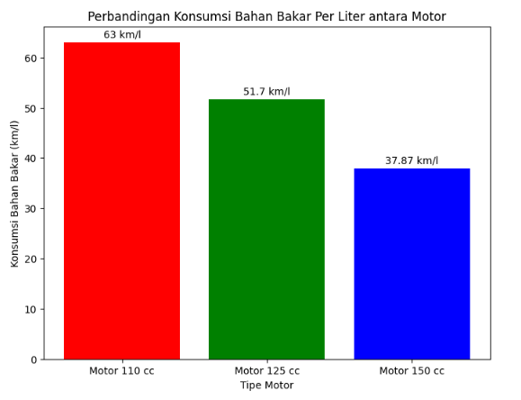
Figure 1. Comparison of fuel consumption per liter on the test vehicle
The selection of these three motorcycle types, representing different vehicle conditions and fuel consumption rates, allows the KNN system to be tested in various scenarios for recommending the nearest gas stations (SPBU) based on the motorcycle type and remaining fuel consumption. This approach illustrates how the KNN system can be applied to vehicles with diverse characteristics, ensuring that the SPBU recommendations are relevant to the varying conditions of different riders. The fuel consumption data used includes various levels of fuel consumption for different engine capacities, ranging from 0.02 to 0.24 liters, which directly influence the prediction process. This fuel consumption data serves as a key feature in the KNN model, helping to determine the predicted travel distance by estimating how far the vehicle can travel with the remaining fuel. The KNN algorithm calculates the distance between the current location of the vehicle and potential gas stations (SPBUs) based on geographic coordinates and remaining fuel. To optimize the model’s performance, several parameters are considered, such as the number of neighbors (K) and the distance metric used to calculate proximity. In this case, the Haversine formula was chosen to calculate the great-circle distance between coordinates, as it accounts for the Earth's curvature and ensures more accurate distance predictions for locations in Surabaya.
The Haversine formula is essential in studies that analyze the distance between two points on the Earth's surface. It provides accurate calculations of the shortest distance between locations based on their geographic coordinates, including latitude and longitude. By considering the curvature of the Earth, the formula ensures realistic distance estimates, especially for long distances. Equation (1) and equation (2) has been widely used and tested in various previous studies, including those in geodesy, navigation, and geographic information systems [30]-[32].
| 
| (1) |
| 
| (2) |
The first formula is used to calculate the value of  , which is the first step in calculating the distance.
  represents the square of the sine, while
  is used to account for the angular difference between the two points on the Earth's surface [33]-[35]. After obtaining the value of , the next step is to calculate the value of
  which is used to convert the angular value into a physical distance that can be calculate with Equation (3).
| 
| (3) |
The  function is a mathematical function that calculates the arc tangent of two values, which are
 and
and  . In this case, the function is used to compute the angle based on the result of . The represents the angle on the Earth's surface between the two points, measured in radians. After calculating the value of , the distance between the two points on the Earth's surface can be determined by multiplying by the Earth's radius (
 ) which is approximately 6.371 km.
| 
| (4) |
In Equation (4),  represents the distance between two points on the Earth's surface (in kilometers, when R is measured in kilometers). After calculating the distance between data points using the Haversine formula, KNN selects the K nearest neighbors by sorting all the calculated distances. K is a pre-determined parameter, set according to the requirements. Once the K nearest neighbors are identified, the next step is to predict the target value for the nearest Gas Station (SPBU) based on the values of the nearest neighbors. The KNN model uses the KNeighborsClassifier from scikit-learn to train a classification model based on location data, specifically latitude and longitude. It also assesses how accessible a particular SPBU is for a vehicle with the remaining fuel capacity. The KNN model is trained by splitting the data into a training set and a testing set using the train_test_split function. After training, the model predicts the class of SPBUs based on their geographic coordinates.
| 
| (5) |
In Equation (5),  represents the predicted value for the point to be predicted.
  denotes the target value of the K nearest neighbors, and K refers to the number of nearest neighbors selected [36]-[40]. Table 1 presents the dataset of locations used for recommending the nearest Gas Stations (SPBUs). This study includes 35 different locations, each with distinct weights based on GPS coordinates and the brand of the SPBU. The distance for each Gas Station and the user's position in Table 1 is calculated using the Haversine formula. The current position of the user is determined to have coordinates of -7.318111111111111, 112.72711111111111. This distance is then used as the KNN dataset to determine the nearest SPBU once the user's remaining fuel reaches a minimum level. Figure 2 displays the map created to facilitate the recognition of coordinate points in the dataset.
Table 1. Dataset system KNN
No. | SPBU | Latitude | Longitude | Distance (Km) | Weight |
1 | Pertamina | -7.311253 | 112.724045 | 0.83 | 0 |
2 | Shell | -7.317313 | 112.747971 | 5.1 | 1 |

|
|
|
|
|
|
35 | BP | -7.273063 | 112.747698 | 5.50 | 2 |
Figure 2. Dataset lokasi SPBU di kota Surabaya
- RESULT
The confusion matrix is used to evaluate how accurately the model classifies Gas Stations (SPBU) into the correct categories, such as PERTAMINA, SHELL, and BP, as shown in Figure 3. The higher the number of True Positive (TP) values in the matrix, the better the model is at predicting the correct class. Conversely, False Positive (FP) and False Negative (FN) values highlight areas that need improvement.
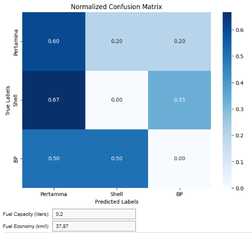
Figure 3. Normalized Confusion Matrix
Several parameters used in classification include precision, recall, F1-score, and accuracy.
| 
| (6) |
Equation (6) represents the measure of accuracy for positive predictions made by the model. Precision measures how many of the predictions made by the model are actually positive. A high precision means the model has few False Positives (incorrect predictions) and many correct predictions for that class. Precision is particularly important in contexts where negative instances are misclassified as positive.
Recall in Equation (7), also known as Sensitivity or True Positive Rate, is a metric that measures the model's ability to detect actual positive instances. Recall evaluates how many positive data points are correctly identified by the model. A high recall indicates that the model successfully captures most of the positive data, with few positive instances missed.
| 
| (7) |
The F1-Score in Equation (8) is the harmonic mean of Precision and Recall. This metric provides a more balanced view between the two, meaning if either of the metrics is low, the F1-Score will also be affected. The F1-Score is particularly useful when there is an imbalance between Precision and Recall. A high F1-Score indicates that the model has both good Precision and Recall in balance. The F1-Score is especially helpful when dealing with imbalanced data (e.g., the number of Shell SPBUs is much smaller than PERTAMINA), as it gives equal weight to both metrics and ensures the model does not overly favor one side (focusing only on Precision or Recall).
| 
| (8) |
Accuracy in Equation (9) is the most commonly used metric to measure the overall correctness of a model's predictions. It calculates the proportion of correct predictions out of the total number of predictions. A high accuracy indicates that the model is able to correctly predict most of the data. However, in this case, a model could have high accuracy simply by predicting most of the data as PERTAMINA, even if its performance in classifying Shell and BP is poor.
| 
| (9) |
The model performs well across all classes (PERTAMINA, SHELL, and BP), as indicated by the provided metrics in Table 2. For PERTAMINA, the model achieves a Precision of 0.80, meaning 80% of the predictions for PERTAMINA are correct, with relatively few False Positives. The Recall is 0.75, indicating that 75% of the actual PERTAMINA instances are correctly detected, but 25% are missed (False Negatives). The F1-Score of 0.77 reflects a balanced performance between Precision and Recall, though there is room to improve the recall to detect more PERTAMINA instances. The Accuracy of 0.80 indicates that the model correctly predicts 80% of the overall data, which is a strong result, though the performance is influenced by the class distribution. For Shell, the model excels, with a Precision of 0.85, meaning 85% of Shell predictions are accurate. The Recall of 0.90 shows that 90% of actual Shell instances are correctly detected, leaving only 10% undetected. The F1-Score of 0.87 indicates a very balanced performance, with both high Precision and Recall. The Accuracy of 0.85 suggests that the model performs consistently well for Shell, making it one of the strongest classes in terms of both detection and correct prediction. For BP, the model also performs well with a Precision of 0.88, indicating that 88% of BP predictions are accurate. The Recall is 0.85, meaning 85% of BP instances are correctly identified. The F1-Score of 0.86 shows a solid balance between Precision and Recall, and the Accuracy of 0.86 indicates that the model performs well for BP, with only a small gap in recall when compared to Shell.
Table 2. Parameter KNN
Merk | Precision | Recall | F1-Score | Accuracy |
PERTAMINA | 0.80 | 0.75 | 0.77 | 0.80 |
SHELL | 0.85 | 0.90 | 0.87 | 0.85 |
BP | 0.88 | 0.85 | 0.86 | 0.86 |
Total |
|
|
| 0.85 |
The Total Accuracy of 0.85 demonstrates that the model correctly predicts 85% of all instances across all classes. This suggests that the model performs well overall, with balanced performance across each class. However, the slightly lower Recall for PERTAMINA suggests that the model could be more sensitive in detecting this class. Overall, the model is highly effective in classifying the different SPBU brands, although there is some room for improvement in specific areas, particularly in detecting PERTAMINA instances.
The KNN model is used to predict the distance to the nearest gas station (SPBU) based on latitude and longitude. The process begins by splitting the data into a training set (67%) and a testing set (33%) using the train_test_split function. The training data is used to train the model, while the testing data is used to evaluate its performance. The KNN model is then tested with various values of K ranging from 1 to 20. For each value of K, the model is trained using the training data and tested on the testing data. Predictions for the distance to the SPBU are generated for the test data, and  is calculated to measure how well the model predicts the distance based on the test data. The value measures how much of the variation in the target data (distance) can be explained by the model.
On the Y-axis, the value in Figure 4 is used to assess how well the model can explain the variability in the predicted target data based on the input features. The value ranges from 0 to 1, with  indicating a perfect model that explains the data variation, while
  means the model is no better than predicting the average. The appropriate R² value depends on the context and purpose of the model. Generally, an value > 0.8 indicates a very good model that explains the data well and makes accurate predictions, which is usually seen with structured data with little noise. values between 0.5 and 0.8 indicate a reasonably good model, although some inaccuracies or patterns remain unexplained, often found in more complex or noisy data. On the other hand, low values < 0.5 suggest that the model is less capable of explaining the data, which can happen if the model is too simplistic or if the data contains a lot of variability that is difficult to predict. For determining the nearest SPBU, an optimal value above 0.6 indicates that the model can explain most of the variation in selecting a relevant SPBU based on the user's location. The K-value on the X-axis in Figure 4 starts at 1 and increases up to 20. As the K-value increases, the model considers more SPBUs, some of which may be farther from the user's location. This can lead to underfitting, as the model becomes less focused on SPBUs that are actually closest to the user. Consequently, a more distant SPBU may be chosen as the nearest one, simply because more neighbors are included in the calculation.
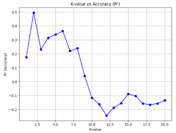
Figure 4. the effect of K-value on accuracy
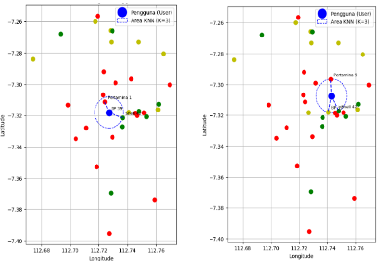
In the graph shown in Figure 5, PERTAMINA SPBUs are marked in red, Shell SPBUs in orange, and BP SPBUs in green. The KNN model (K=3) searches for the three nearest SPBUs from the user's location, represented by the blue circle. The distance between the user's point (the blue dot) and the SPBUs within the blue circle provides an indication of how close the chosen SPBU is to the user's location. The smaller the distance between the user and the SPBU, the more accurate the model is in selecting the nearest SPBU. The number of SPBUs within the blue circle is also important, as it represents the density of SPBUs around the user. If many SPBUs are within this area, the model has more options to choose from, making the selection more accurate. Conversely, if there are only a few SPBUs in the area, the model’s decision will be more limited. The colors of the SPBUs (red for PERTAMINA, yellow for Shell, and green for BP) indicate their proximity to the user. Red SPBUs (PERTAMINA) are likely farther from the user and become the furthest neighbor in the nearest neighbors set, while BP SPBUs (green) tend to be closer and may be more relevant for selection as the nearest SPBU. Shell SPBUs (yellow) might be in between, farther than BP but closer than PERTAMINA.
The density of SPBUs around the user also affects the efficiency of the SPBU selection. When many SPBUs are nearby, the KNN model will be more efficient in selecting the truly nearest SPBU. However, if the SPBUs are spread out over a large area, the model may select a farther SPBU, which could reduce the prediction accuracy in the context of determining the nearest SPBU location.
Figure 5. The KNN model predicts the distance with K=3 and detects the nearest SPBU
Figure 6 presents the final results of the prediction system that calculates the distance to the nearest Gas Station (SPBU) based on the vehicle's remaining fuel condition. At the top, there is information about the Maximum Distance That Can Be Traveled with Remaining Fuel, which is calculated as 3.79 km, indicating how far the vehicle can travel with the available fuel. The Predicted Nearest Distance is 3.11 km, which shows the closest SPBU that can be reached based on the remaining fuel. The displayed Predicted Nearest Distance is the value generated by the KNN model, based on the data of remaining fuel capacity and fuel consumption per liter. In this case, the KNN model calculates the distance between the user's location and the nearest SPBUs around them, taking into account geographical data. By using the KNN model, the system estimates the nearest SPBU that the vehicle can reach, based on the user's location and the distance to the nearest SPBU points. The 3.11 km listed as the Predicted Nearest Distance is the result of KNN's calculation, projecting the distance to the closest SPBU while considering the vehicle's fuel condition and capacity. The KNN model uses coordinate data to select the three nearest SPBUs (K=3), and this distance is used to estimate which SPBU is accessible with the remaining fuel, providing users with a more accurate prediction of the distance they need to travel. Additionally, there is information about the distance to Tanjung Perak Port, which is 10.71 km, offering additional context for potential longer trips. The bottom section of the display shows a list of the nearest SPBUs with the Predicted Distance, where for each SPBU, the name, address, distance to the user's location, and estimated remaining fuel after reaching the SPBU are displayed. This provides a clear overview of which SPBUs are the closest and how much fuel will remain after the trip, allowing users to plan their journey more efficiently and effectively.
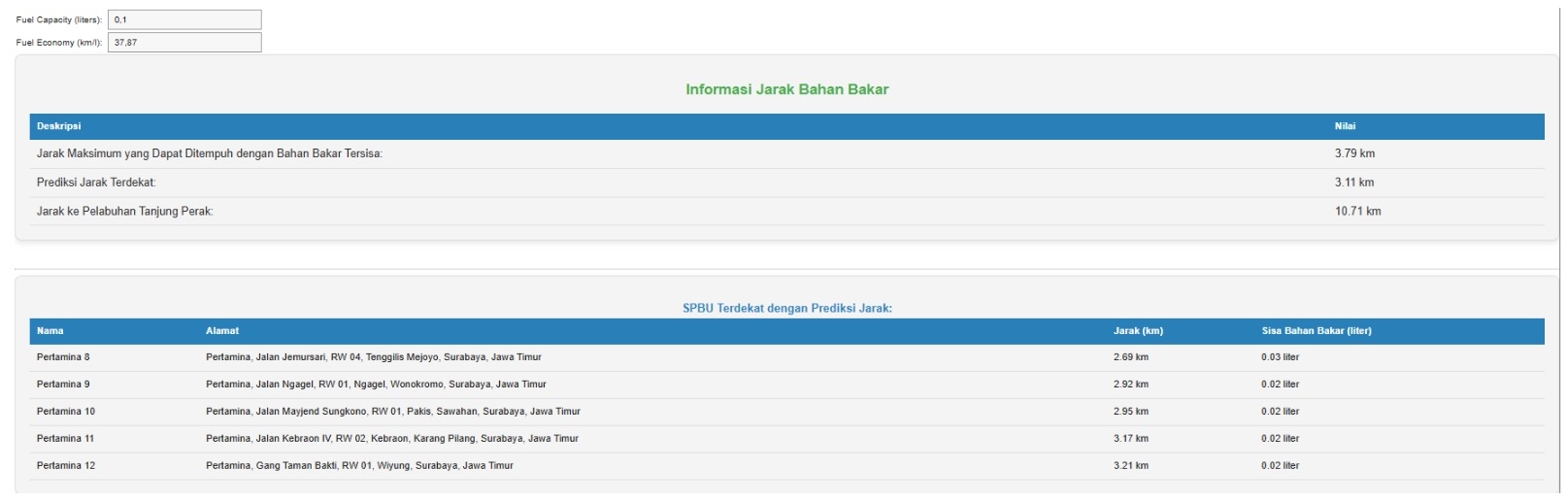
Figure 6. User interface system
As the distance a vehicle can travel increases, the predicted travel distance provided by the model tends to show a saturation or limitation. This is related to the constraints of the available dataset, particularly in terms of the distance that can be covered by the vehicle based on the amount of fuel remaining. In the context of the given dataset, it can be observed that at higher fuel consumption rates (e.g., 0.24), the recorded distances that the vehicle can travel are greater, such as 15.12 km, 12.41 km, and 9.09 km. However, despite the increasing recorded distance, the predictions made by the K-Nearest Neighbors (KNN) model show results that tend to stabilize and even saturate at 7.56 across all categories. This saturation occurs due to several key factors, one of which is the limitation on the distance that can be reached by the Gas Stations (SPBUs) available in the dataset. In this case, the prediction system may have already assumed a constraint on the maximum distance that can be traveled before the vehicle reaches the nearest SPBU, which limits the distance further even though the vehicle has enough fuel.
In other words, even though the remaining fuel allows the vehicle to travel a longer distance, the prediction system converges to a certain value that cannot exceed the distance limitation before the driver needs to refuel at the nearest SPBU. This indicates that the model cannot fully predict further distances due to practical factors that limit it, such as the geographic location and the coverage of SPBUs present in the dataset. Therefore, even as fuel consumption decreases, the predicted travel distance will stop or saturate at a certain point due to the limitations of the system. The differences in the graphs for each engine type can be seen in Figure 7, Figure 8, and Figure 9. To validate the system, MAE (Mean Absolute Error) and MAPE (Mean Absolute Percentage Error) calculations are used [41]-[47].
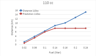
Figure 7. Comparison of actual distance vs predicted distance in a 110cc engine
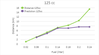
Figure 8. Comparison of actual distance vs predicted distance in a 125cc engine
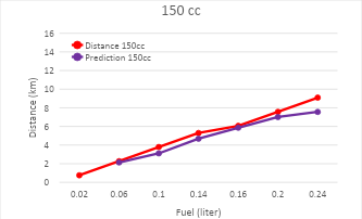
Figure 9. Comparison of actual distance vs predicted distance in a 150cc engine
The results in Table 3 show that at a fuel consumption level of 0.06 liters, the RMSE is recorded at 0.4086, indicating the lowest prediction error. This suggests that the model provides the most accurate predictions at lower fuel consumption levels. Next, at a fuel consumption of 0.02 liters, the RMSE slightly increases to 0.4024, although still relatively low, indicating that the prediction error is slightly larger but remains within a good accuracy range. At a fuel consumption of 0.10 liters, the RMSE rises to 0.5436, which is still relatively low, indicating that the model continues to provide reasonably accurate predictions, despite a slight decline in accuracy compared to the lower consumption levels. However, at a fuel consumption of 0.14 liters, the RMSE increases to 0.8191, showing a rise in prediction error. The model begins to struggle with making accurate predictions at higher fuel consumption levels. At a fuel consumption of 0.16 liters, the RMSE increases significantly to 1.6307, indicating a noticeable decline in prediction accuracy as fuel consumption increases. Moving to a consumption level of 0.20 liters, the RMSE sharply rises to 3.3388, reflecting much larger prediction errors. The model becomes increasingly inaccurate in predicting vehicle travel distance at higher fuel consumption rates. Finally, at a fuel consumption of 0.24 liters, the RMSE reaches the highest value of 5.2605, indicating a significant prediction error. This suggests that the model performs very poorly at very high fuel consumption levels, and the prediction error increases drastically as consumption rises.
Table 3. KNN Final Result
Fuel Consumption (Liter) | MAE | MAPE (%) | RMSE |
0.02 | 0.347 | 31.21 | 0.40 |
0.06 | 0.330 | 9.90 | 0.41 |
0.10 | 0.533 | 11.40 | 0.54 |
0.14 | 0.700 | 9.66 | 0.82 |
0.16 | 1.327 | 14.51 | 1.63 |
0.20 | 2.793 | 24.76 | 3.34 |
0.24 | 4.647 | 35.30 | 5.26 |
- CONCLUSION
Based on the results from applying the K-Nearest Neighbors (KNN) algorithm, the model shows excellent performance at low fuel consumption levels. At a consumption of 0.02 liters, with a MAPE of 31.21%, but an MAE of only 0.347 and a small RMSE of 0.40, the prediction error is overall very small, indicating that the model provides quite accurate predictions. Similarly, at a fuel consumption of 0.06 liters, with a MAPE of just 9.90% and a slightly higher RMSE of 0.41, the KNN model proves to be highly effective in predicting vehicle travel distances with good accuracy at higher fuel consumption levels. This success is also reflected in other fuel consumption levels, such as 0.10 liters and 0.14 liters, where prediction errors remain within an acceptable range, with relatively low MAPE and RMSE values. This demonstrates that the KNN model is highly capable of handling various fuel consumption rates, providing accurate and consistent distance predictions.
The results suggest that the KNN model can be reliably used in predicting travel distances based on fuel consumption. It is particularly effective at lower consumption rates, making it ideal for applications that require real-time, low-energy predictions, such as in navigation systems and fleet management. The model's ability to maintain accuracy at higher fuel consumption levels also opens up possibilities for broader usage in different types of vehicles with varying fuel efficiencies. In Surabaya, the limited number of gas stations and their uneven distribution pose a major challenge. This makes the prediction and recommendation of the nearest gas stations less effective when the vehicle still has a significant amount of fuel, as the system cannot provide accurate recommendations for longer trips with sufficient fuel.
Future work could explore expanding the model's capabilities by incorporating additional variables such as traffic data, road conditions, and vehicle load, which could further refine the distance predictions. Investigating alternative algorithms, such as support vector machines (SVM) or deep learning models, could also provide insights into whether these approaches can improve prediction accuracy, especially for more complex datasets or high-consumption scenarios. Additionally, integrating real-time data from IoT devices could further enhance the model's performance and make it more adaptive to dynamic driving conditions.
REFERENCES
- Y. Chen et al., “Fast density peak clustering for large scale data based on kNN,” Knowledge-Based Syst., vol. 187, p. 104824, 2020, https://doi.org/10.1016/j.knosys.2019.06.032.
- D. Xu, Y. Wang, P. Peng, S. Beilun, Z. Deng, and H. Guo, “Real-time road traffic state prediction based on kernel-KNN,” Transp. A Transp. Sci., vol. 16, no. 1, pp. 104–118, 2020, https://doi.org/10.1080/23249935.2018.1491073.
- J. Miao, Y. Liu, Q. Yin, G. Zhang, and Y. Yuan, “Research on the Influence of Signal Sampling Frequency on Soft Fault Diagnosis Accuracy of DC/DC Converters,” CPSS Trans. Power Electron. Appl., vol. 8, no. 1, pp. 33–41, 2023, https://doi.org/10.24295/CPSSTPEA.2023.00004.
- O. Kherif, Y. Benmahamed, M. Teguar, A. Boubakeur, and S. S. M. Ghoneim, “Accuracy Improvement of Power Transformer Faults Diagnostic Using KNN Classifier With Decision Tree Principle,” IEEE Access, vol. 9, pp. 81693–81701, 2021, https://doi.org/10.1109/ACCESS.2021.3086135.
- E. A. Hassan, A. M. Mohamed, F. A. Eltaib, A. M. S. Khaled, and et al., “Determinants of Nursing Students’ Satisfaction with Blended Learning,” BMC Nurs., vol. 23, no. 1, p. 766, 2024, https://doi.org/10.1186/s12912-024-02393-y.
- S. Uddin, I. Haque, H. Lu, M. A. Moni, and E. Gide, “Comparative performance analysis of K-nearest neighbour (KNN) algorithm and its different variants for disease prediction,” Sci. Rep., vol. 12, no. 1, p. 6256, 2022, https://doi.org/10.1038/s41598-022-10358-x.
- S. Zhang, “Cost-sensitive KNN classification,” Neurocomputing, vol. 391, pp. 234–242, 2020, https://doi.org/https://doi.org/10.1016/j.neucom.2018.11.101.
- L. Xiong and Y. Yao, “Study on an adaptive thermal comfort model with K-nearest-neighbors (KNN) algorithm,” Build. Environ., vol. 202, p. 108026, 2021, https://doi.org/10.1016/j.buildenv.2021.108026.
- H. Durani, M. Sheth, M. Vaghasia, and S. Kotech, “Smart Automated Home Application using IoT with Blynk App,” Proc. Int. Conf. Inven. Commun. Comput. Technol. ICICCT 2018, pp. 393–397, 2018, https://doi.org/10.1109/ICICCT.2018.8473224.
- N. Ukey, Z. Yang, B. Li, G. Zhang, Y. Hu, and W. Zhang, “Survey on Exact kNN Queries over High-Dimensional Data Space,” Sensors, vol. 23, no. 2, 2023, https://doi.org/10.3390/s23020629.
- S. Zhang, “Challenges in KNN Classification,” IEEE Trans. Knowl. Data Eng., vol. 34, no. 10, pp. 4663–4675, 2022, https://doi.org/10.1109/TKDE.2021.3049250.
- S. Zhang and J. Li, “KNN Classification With One-Step Computation,” IEEE Trans. Knowl. Data Eng., vol. 35, no. 3, pp. 2711–2723, 2023, https://doi.org/10.1109/TKDE.2021.3119140.
- H. Lee, H. Choi, K. Sohn, and D. Min, “KNN Local Attention for Image Restoration,” in 2022 IEEE/CVF Conference on Computer Vision and Pattern Recognition (CVPR), pp. 2129–2139, 2022, https://doi.org/10.1109/CVPR52688.2022.00218.
- S. Goyal, “Handling Class-Imbalance with KNN (Neighbourhood) Under-Sampling for Software Defect Prediction,” Artif. Intell. Rev., vol. 55, no. 3, pp. 2023–2064, 2022, https://doi.org/10.1007/s10462-021-10044-w.
- K. Kim, “Normalized class coherence change-based kNN for classification of imbalanced data,” Pattern Recognit., vol. 120, p. 108126, 2021, https://doi.org/https://doi.org/10.1016/j.patcog.2021.108126.
- Sukamto, Hadiyanto, and Kurnianingsih, “KNN Optimization Using Grid Search Algorithm for Preeclampsia Imbalance Class,” E3S Web Conf., vol. 448, p. 2057, 2023, https://doi.org/10.1051/e3sconf/202344802057.
- Z. Lei, L. Zhu, Y. Fang, X. Li, and B. Liu, “Anomaly detection of bridge health monitoring data based on KNN algorithm,” J. Intell. \& Fuzzy Syst., vol. 39, no. 4, pp. 5243–5252, 2020, https://doi.org/10.3233/JIFS-189009.
- B. S. Yaswanth, “Smart Safety and Security Solution for Women using kNN Algorithm and IoT,” no. i, pp. 87–92, 2020, https://doi.org/10.1109/MPCIT51588.2020.9350431.
- A. Ali, M. A. T. Alrubei, L. F. M. Hassan, M. A. M. Al-Ja’afari, and S. H. Abdulwahed, “Diabetes Diagnosis Based On Knn,” IIUM Eng. J., vol. 21, no. 1, pp. 175–181, 2020, https://doi.org/10.31436/iiumej.v21i1.1206.
- A. Juna et al., “Water Quality Prediction Using KNN Imputer and Multilayer Perceptron,” Water, vol. 14, no. 17, 2022, https://doi.org/10.3390/w14172592.
- W. Zhuang and Y. Cao, “Short-Term Traffic Flow Prediction Based on a K-Nearest Neighbor and Bidirectional Long Short-Term Memory Model,” Appl. Sci., vol. 13, no. 4, 2023, https://doi.org/10.3390/app13042681.
- J. Jang, “Travel time prediction using machine learning algorithms: focusing on k-NN, LSTM, and Transformer,” The Open Transportation Journal, vol. 18, no. 1, 2024, https://doi.org/10.2174/0126671212356139241101070347.
- A. F. Aritenang, S. R. Ginting, and A. D. Sakti, “Metropolitan spatial structure based on commuting pattern: a comparison between Jakarta and Surabaya metropolitans,” International Journal of Urban Sciences, vol. 29, no. 2, pp. 503-521, 2025, https://doi.org/10.1080/12265934.2024.2358101.
- G. N. A. Pranoto, A. Jatayu, M. R. I. Robbik, R. Hamdika, and N. Nurjannah, “Sensitivity of Variables Affecting Urban Heat Island (UHI) Intensity to Different Levels of Transit Oriented Development (TOD) and Non TOD-Adjacent Areas in Jakarta City,” In IOP Conference Series: Earth and Environmental Science, vol. 1498, no. 1, p. 012009, 2025, https://doi.org/10.1088/1755-1315/1498/1/012009.
- R. A. Nugraha and R. Christiawan, “Airport Development in Indonesia: Legal and Policy Considerations,” In Aerodrome Governance in Asia: Legal and Managerial Perspectives, pp. 139-157, 2025, https://doi.org/10.1007/978-981-96-7568-5_8.
- Y. K. Thakre and P. Y. Pawade, “Traffic Congestion at Urban Road-Review,” In IOP Conference Series: Earth and Environmental Science, vol. 1326, no. 1, p. 012094, 2024, https://doi.org/10.1088/1755-1315/1326/1/012094.
- N. T. Tuan and N. P. Dong, “Improving performance and reducing emissions from a gasoline and liquefied petroleum gas bi-fuel system based on a motorcycle engine fuel injection system,” Energy for Sustainable Development, vol. 67, pp. 93-101, 2022, https://doi.org/10.1016/j.esd.2022.01.010.
- R. Lopes et al., “Passive Safety Solutions on Coach according ECE R29: Experimental and Numerical analyses,” Procedia Struct. Integr., vol. 42, pp. 1159–1168, 2022, https://doi.org/10.1016/j.prostr.2022.12.148.
- Y. Liu, Y. G. Liao, and M. C. Lai, “Effects of battery pack capacity on fuel economy of hybrid electric vehicles,” In 2021 IEEE Transportation Electrification Conference & Expo (ITEC), pp. 771-775, 2021, https://doi.org/10.1109/ITEC51675.2021.9490040.
- R. A. Azdy and F. Darnis, “Use of Haversine Formula in Finding Distance Between Temporary Shelter and Waste End Processing Sites,” J. Phys. Conf. Ser., vol. 1500, no. 1, p. 12104, 2020, https://doi.org/10.1088/1742-6596/1500/1/012104.
- E. Maria, E. Budiman, Haviluddin, and M. Taruk, “Measure distance locating nearest public facilities using Haversine and Euclidean Methods,” J. Phys. Conf. Ser., vol. 1450, no. 1, p. 12080, 2020, https://doi.org/10.1088/1742-6596/1450/1/012080.
- D. Ikasari, Widiastuti, and R. Andika, “Determine the Shortest Path Problem Using Haversine Algorithm, A Case Study of SMA Zoning in Depok,” in 2021 3rd International Congress on Human-Computer Interaction, Optimization and Robotic Applications (HORA), 2021, pp. 1–6. https://doi.org/10.1109/HORA52670.2021.9461185.
- S. A. Ige, M. S. Khan, and B. R. Biju, “Enhancing EV Charging Capabilities Using Haversine and Convex Optimization for ITS,” in 2023 IEEE Virtual Conference on Communications (VCC), 2023, pp. 165–170. https://doi.org/10.1109/VCC60689.2023.10475040.
- A. Andreou, C. X. Mavromoustakis, J. M. Batalla, E. K. Markakis, G. Mastorakis, and S. Mumtaz, “UAV Trajectory Optimisation in Smart Cities Using Modified A* Algorithm Combined With Haversine and Vincenty Formulas,” IEEE Trans. Veh. Technol., vol. 72, no. 8, pp. 9757–9769, 2023, https://doi.org/10.1109/TVT.2023.3254604.
- B. Işik, “Area Optimized FPGA Implementation of Slant Range Calculation Using Haversine Formula,” in 2021 29th Signal Processing and Communications Applications Conference (SIU), 2021, pp. 1–4. https://doi.org/10.1109/SIU53274.2021.9478008.
- Z. Bian, C. M. Vong, P. K. Wong, and S. Wang, “Fuzzy KNN Method With Adaptive Nearest Neighbors,” IEEE Trans. Cybern., vol. 52, no. 6, pp. 5380–5393, 2022, https://doi.org/10.1109/TCYB.2020.3031610.
- N. Marchang and R. Tripathi, “KNN-ST: Exploiting Spatio-Temporal Correlation for Missing Data Inference in Environmental Crowd Sensing,” IEEE Sens. J., vol. 21, no. 3, pp. 3429–3436, 2021, https://doi.org/10.1109/JSEN.2020.3024976.
- A. Pérez-Navarro, R. Montoliu, E. Sansano-Sansano, M. Martínez-Garcia, R. Femenía, and J. Torres-Sospedra, “Accuracy of a Single Position Estimate for kNN-Based Fingerprinting Indoor Positioning Applying Error Propagation Theory,” IEEE Sens. J., vol. 23, no. 16, pp. 18765–18775, 2023, https://doi.org/10.1109/JSEN.2023.3287856.
- C. Lin and N. D. Doyog, “Applying a Four-Way Factorial Experimental Model to Diagnose Optimum kNN Parameters for Precise Aboveground Biomass Mapping,” IEEE J. Sel. Top. Appl. Earth Obs. Remote Sens., vol. 18, pp. 479–495, 2025, https://doi.org/10.1109/JSTARS.2024.3486737.
- I. G. S. M. Diyasa, D. A. Prasetya, M. Idhom, A. P. Sari, and A. M. Kassim, “Implementation of Haversine Algorithm and Geolocation for travel recommendations on Smart Applications for Backpackers in Bali,” in 2022 International Conference on Informatics, Multimedia, Cyber and Information System (ICIMCIS), pp. 504–508, 2022, https://doi.org/10.1109/ICIMCIS56303.2022.10017760.
- Y. Li, S. Guo, G. Ma, Z. Li, J. Yang, and Z. Chen, “Dynamic Estimation of Load-Side Equivalent Inertia by Using Clustering Method,” CPSS Trans. Power Electron. Appl., vol. 10, no. 1, pp. 1–9, 2025, https://doi.org/10.24295/CPSSTPEA.2025.00001.
- Y. Chen, Z. Shen, Z. Xu, L. Jin, and W. Chen, “Parameter Shift Prediction of Planar Transformer Based on Bi-LSTM Algorithm,” CPSS Trans. Power Electron. Appl., vol. 8, no. 1, pp. 13–22, 2023, https://doi.org/10.24295/CPSSTPEA.2023.00002.
- M. Slawski, E. Ben-David, and P. Li, “Two-stage approach to multivariate linear regression with sparsely mismatched data,” J. Mach. Learn. Res., vol. 21, no. 204, pp. 1-42. 2020, https://www.jmlr.org/papers/v21/19-645.html.
- Y. Quan, C. Liu, Z. Yuan, and Y. Zhou, “An Intelligent Multiscale Spatiotemporal Fusion Network Model for TCM,” IEEE Sens. J., vol. 23, no. 7, pp. 6628–6637, 2023, https://doi.org/10.1109/JSEN.2023.3244587.
- S. Mishra, P. K. Mallick, H. K. Tripathy, L. Jena, and G.-S. Chae, “Stacked KNN with hard voting predictive approach to assist hiring process in IT organizations,” Int. J. Electr. Eng. \& Educ., vol. 0, no. 0, p. 0020720921989015, https://doi.org/10.1177/0020720921989015.
- E. Sitompul, R. M. Putra, H. Tarigan, A. Silitonga, and I. Bukhori, “Implementation of Digital Feedback Control with Change Rate Limiter in Regulating Water Flow Rate Using Arduino,” Bul. Ilm. Sarj. Tek. Elektro, vol. 6, no. 1, pp. 72–82, 2024, https://doi.org/10.12928/biste.v6i1.10234.
- H. D. Trung, “Estimation of Crowd Density Using Image Processing Techniques with Background Pixel Model and Visual Geometry Group,” Bul. Ilm. Sarj. Tek. Elektro, vol. 6, no. 2, pp. 142–154, 2024, https://doi.org/10.12928/biste.v6i2.10785.
AUTHOR BIOGRAPHY

| Farid Baskoro is a lecturer at Surabaya State University. In the past 5 years, he has taught 47 courses. He has conducted 12 community service activities. He has published 93 scientific articles in journals. He has authored 1 book. He has been a speaker at 6 scientific seminars. He has obtained 1 intellectual property right (IPR). Email: faridbaskoro@unesa.ac.id |
|
|

| Widi Aribowo is a lecturer at Surabaya State University. In the past 5 years, he has taught 43 courses. He has conducted 14 community service activities. He has published 185 scientific articles in journals. He has authored 3 books. He has been a speaker at 14 scientific seminars. He has obtained 14 intellectual property rights (IPR). Email: widiaribowo@unesa.ac.id |
|
|

| Hisham Shehadeh obtained his Ph.D. from Department of Computer System and Technology, University of Malaya, Kuala Lumpur, Malaysia in 2018. He worked as a Lecturer in the CS Department at the College of Computer and Information Technology, Jordan University of Science and Technology, Irbid, Jordan. He received his M.S. degree in computer science from Jordan University of Science and Technology, Irbid, Jordan in 2014. He obtained his B.S. degree in computer science from Al-Balqa` Applied University, As-Salt, Jordan, in 2012. His current research interests are algorithmic engineering applications of wireless sensor networks, artificial intelligence, and computing. Email: h.shehadeh@aau.edu.jo |
|
|
| Hewa Majeed Zangana is an Assistant Professor currently affiliated with Duhok Polytechnic University (DPU) in Iraq. He holds a Doctorate in Philosophy (PhD) degree in ITM, which he is currently pursuing at DPU. Prior to his current role, Hewa Majeed Zangana has held various academic and managerial positions. He previously served as an Assistant Professor at Ararat Private Technical Institute and a Lecturer at DPU's Amedi Technical Institute, and Nawroz University. He has also held administrative positions such as Curriculum Division Director - Presidency of DPU, Information Unit Manager of The Research Center at Duhok Polytechnic University, Head of the Computer Science Department at Nawroz University, and Acting Dean of the College of Computer and IT at Nawroz University. Hewa Majeed Zangana's research interests span a wide range of topics in computer science, including network systems, information security, mobile communication, data communication, and intelligent systems. Email: hewa.zangana@dpu.edu.krd |
|
|

| Wahyu Sasongko Putro is a proactive individual with strong analytical skills and extensive experience in the field of Space Science (atmospheric studies). He has written several journal articles and book chapters (indexed in Scopus) on Thunderstorm modeling using Artificial Intelligence, such as Artificial Neural Networks (ANN), Fuzzy Logic, and Adaptive Neuro-Fuzzy Inference Systems (ANFIS). Email: wahyusas001@e.ntu.edu.sg |
|
|

| Sri Dwiyanti is a lecturer at Surabaya State University. In the past 5 years, she has taught 23 courses. She has conducted 15 community service activities. She has published 154 scientific articles in journals. She has authored 1 book. He has obtained 7 intellectual property rights (IPR). Email: sridwiyanti@unesa.ac.id |
|
|

| Aristyawan Putra Nurdiansyah is a researcher and academic affiliated with the Department of Electrical Engineering at Surabaya State University (UNESA), Indonesia. He is involved in the fields of electrical engineering, control systems, and emerging technologies such as the Internet of Things (IoT) and sensor networks. He has published 15 scientific articles in journals and has obtained 1 intellectual property right (IPR). Email: aristyawannurdiansyah@mhs.unesa.ac.id |
Farid Baskoro (K-Nearest Neighbors for Smart Solution Transportation: Prediction Distance Travel and Optimization of Fuel Usage and Charging Recommendations for ICE Vehicles Based in Surabaya)