ISSN: 2685-9572 Buletin Ilmiah Sarjana Teknik Elektro
Vol. 7, No. 4, December 2025, pp. 993-1012
Hybrid Bayesian–Hyperband Optimization of a One-Dimensional Convolutional Neural Network for Short-Term Load Forecasting
Trung Dung Nguyen, Nguyen Anh Tuan
FEET, Industrial University of Ho Chi Minh City, Ho Chi Minh City, Viet Nam
ARTICLE INFORMATION |
| ABSTRACT |
Article History: Received 28 September 2025 Revised 11 December 2025 Accepted 23 December 2025 |
| 
Short-term load forecasting (STLF) plays a crucial role in power system operation and electricity market planning. However, the forecasting accuracy of convolutional neural network (CNN) models strongly depends on properly tuned hyperparameters such as filter numbers, batch size, and loss function, while exhaustive tuning is computationally expensive. This paper proposes a one-dimensional CNN (1D-CNN) for STLF whose key hyperparameters are optimized by a hybrid Bayesian Optimization–Hyperband framework (BO-TPE-HB). The framework combines the Tree-structured Parzen Estimator (TPE), which guides the search towards promising regions of the hyperparameter space, with Hyperband’s multi-fidelity early-stopping strategy to terminate weak configurations early and save computation. The proposed approach is evaluated using half-hourly electricity load data from the Australian Energy Market Operator (AEMO) for New South Wales (NSW) and Victoria (VIC) from 2009 to 2014. Using a rolling-origin time-series cross-validation scheme on the training set and a chronologically separated hold-out test set, BO-TPE-HB explores 100 candidate configurations of a 4-layer 1D-CNN with a sliding window of 48 time steps. Model performance is assessed using MAE, MSE, RMSE, MAPE, and total hyperparameter optimization runtime. Experimental results show that the BO-TPE-HB–tuned CNN achieves test MAPE of 1.350% (MAE 105.98 MW, RMSE 143.71 MW) for NSW and 1.615% (MAE 89.13 MW, RMSE 124.25 MW) for VIC, outperforming Random Search, standalone TPE, and standalone Hyperband in terms of both prediction accuracy and computational efficiency, while requiring substantially less tuning time than plain Bayesian Optimization. These findings highlight that combining probabilistic search with resource-efficient early stopping provides a practical and reproducible way to enhance CNN-based STLF, and can be extended to multivariate inputs or other deep learning forecasting architectures in future work. |
Keywords: Short-Term Load Forecasting; Hyperparameter Optimization; Bayesian Optimization; Hyperband; Optuna; TimeSeriesSplit; 1D-CNN |
Corresponding Author: Nguyen Anh Tuan,
FEET, Industrial University of Ho Chi Minh City, Ho Chi Minh City, Viet Nam.
Email: nguyenanhtuan@iuh.edu.vn |
This work is licensed under a Creative Commons Attribution-Share Alike 4.0 
|
Document Citation: T. D. Nguyen and N. A. Tuan, “Hybrid Bayesian–Hyperband Optimization of a One-Dimensional Convolutional Neural Network for Short-Term Load Forecasting,” Buletin Ilmiah Sarjana Teknik Elektro, vol. 7, no. 4, pp. 993-1012, 2025, DOI: 10.12928/biste.v7i4.14824. |
- INTRODUCTION
Short-term load forecasting (STLF) is a key element in the operation and planning of modern power systems. Accurate near-term demand forecasts enable the optimization of generation scheduling, reduction of operating costs, and improvement of grid reliability. Traditional forecasting methods include linear regression [1]-[4], moving averages [5],[6], ARIMA [7]-[11], and support vector regression [12]-[16]. However, these models cannot capture nonlinear patterns and short-term fluctuations in half-hourly (30-minute) load data. In recent years, deep learning models—including Multi-Layer Perceptrons (MLPs) [17]-[20], Long Short-Term Memory (LSTM) networks [21]-[28], and Convolutional Neural Networks (CNNs) [29]-[37]—have demonstrated strong potential for time-series forecasting. In particular, CNNs effectively extract local features from sequential data, making them well-suited to represent daily and weekly regularities in STLF. Despite this promise, achieving high accuracy in STLF requires careful selection of hyperparameters [38]-[44]. Hyperparameters, including the number of convolutional filters per layer, learning rate, batch size, loss function, and the number of training epochs, strongly influence CNN performance. Selecting these hyperparameters manually or through trial and error is difficult due to the ample search space and complex interactions among hyperparameters. We focus on these particular hyperparameters because they directly control model capacity (the number of filters per layer), optimization dynamics (learning rate, batch size, and maximum number of epochs), and error sensitivity (the loss function). In contrast, other parameters (e.g., kernel size or optimizer choice) are fixed based on preliminary experiments and standard best practices to keep the search space tractable.
A common approach is to apply single-stage hyperparameter optimization over the whole search space. Popular techniques include Grid Search [45]-[50], Random Search [51]-[54], Bayesian Optimization (BO) [55]-[68], and evolutionary algorithms, genetic algorithms [69][70]. Random Search is widely used for simplicity and often outperforms Grid Search in high-dimensional spaces. BO leverages probabilistic surrogate models to find better configurations with fewer evaluations than random search; it can converge to good settings faster and with fewer trials—an advantage when training is costly. However, single-stage approaches face challenges: pure Random Search may waste resources on unpromising trials, while vanilla BO spends time modeling the objective and, with few observations, can behave similarly to random search. Moreover, these methods often struggle to balance exploration and exploitation in high-dimensional, multimodal spaces, risking local optima or missing the global optimum under limited budgets.
Multi-fidelity and hybrid optimization strategies have been proposed to address these issues. A representative method is Hyperband—a bandit-based hyperparameter optimizer that dynamically allocates training resources and uses successive halving to early discard poor configurations [71][72]. Hyperband offers strong anytime performance and scalability by evaluating numerous configurations with limited budgets, while only a few are reviewed with the full budget. Its drawback is that configurations are selected randomly, and it does not learn from past evaluations, which can reduce final accuracy compared with model-based search. Conversely, model-based BO methods such as the Tree-structured Parzen Estimator (TPE) build probabilistic models of “good” vs. “bad” hyperparameters to guide search toward promising regions. Yet, conventional BO (without multi-fidelity) evaluates all trials using the entire training budget, which is computationally expensive for deep models.
Research gap and motivation. Existing CNN-based STLF studies typically (i) rely on single-stage hyperparameter optimization (Grid/Random/TPE/GA) or (ii) assess Hyperband in isolation, and thus pay limited attention to a model-guided, multi-fidelity strategy that jointly optimizes forecasting accuracy and tuning time under realistic computational budgets. To the best of our knowledge, a systematic assessment of a BO-TPE-HB framework for CNN-based STLF on real electricity-market data—under a unified and reproducible evaluation protocol—has not been reported. This study makes three main contributions:
- We propose a BO-TPE-HB-based pipeline for CNN hyperparameter tuning in STLF, combining TPE-based probabilistic search with Hyperband’s multi-fidelity dynamic resource allocation.
- We design and adopt a reproducible evaluation protocol on half-hourly (30-minute) AEMO load data for New South Wales (NSW) and Victoria (VIC) over 2009–2014, using MAE/MSE/RMSE/MAPE together with total tuning time as joint criteria, and demonstrate that the BO-TPE-HB–tuned CNN can achieve a test MAPE of about 1.0% while reducing tuning time compared with conventional BO.
- We provide a comprehensive comparison against Random Search, TPE, and Hyperband, showing that BO-TPE-HB offers the best overall trade-off between forecasting accuracy and computational efficiency among the considered hyperparameter-tuning methods.
Problem setting and scope. We study univariate half-hourly load forecasting in a sliding-window formulation, with a look-back length of  (in 30-minute increments) and a horizon of
  (in 30-minute increments). The default setting is
  step (30 minutes ahead). Unless otherwise noted, we use
  steps to provide a 24-hour context (and
  steps for a 7-day context when analyzing weekly patterns). No exogenous variables are included; model selection uses time-series cross-validation, and final performance is reported on a held-out test set. The datasets comprise real half-hourly electricity-load series from NSW and VIC (AEMO, 2009–2014). This univariate setup enables us to isolate the impact of hyperparameter optimization on the CNN architecture itself; incorporating exogenous variables, such as weather or calendar features, is left for future work.
This paper employs the hybrid optimizer BO-TPE-HB to tune CNN hyperparameters for STLF. BO-TPE-HB unifies the strengths of Bayesian optimization and Hyperband, utilizing BO’s probabilistic modeling to guide the search toward promising regions. It applies Hyperband’s dynamic resource allocation (successive halving) to manage compute efficiently. The rationale is that BO-TPE-HB can better balance exploration and exploitation, finding high-performing configurations faster than standard BO and yielding superior final results to Hyperband alone. We evaluate BO-TPE-HB for STLF and compare it with traditional hyperparameter-tuning methods. We optimize a CNN on real load datasets from two regions (NSW and VIC) and assess forecasting accuracy (MAE, MSE, RMSE, MAPE) and tuning time for each method. In summary, the research contribution of this work is a hybrid BO-TPE-HB hyperparameter optimization framework for CNN-based STLF, along with its thorough validation against state-of-the-art tuning strategies on real AEMO load data. The remainder of this paper is organized as follows: Section II describes the proposed BO-TPE-HB-based CNN model and experimental protocol; Section III presents the results and discussion; and Section IV concludes the paper with key findings and directions for future work.
- PROPOSED METHOD
- CNN Model Architecture for STLF
We design a convolutional neural network (CNN) specifically tailored for the short-term load forecasting problem, using historical load sequences as input to predict the load value at the next 30-minute step. The CNN takes as input a one-dimensional sequence of past load values. In our implementation, we use the previous 48 steps (24 hours, corresponding to 1 day) as input features, represented as (48, 1) for each sample (48 time steps, one feature). This univariate configuration allows us to isolate and analyze the impact of hyperparameter optimization on the CNN architecture itself.
The base CNN architecture consists of four one-dimensional convolutional (Conv1D) layers arranged in sequence, with an increasing number of filters. In the initial baseline design, we use (16, 32, 64, 128) filters for the four layers, respectively; however, in the proposed framework, these filter values are not kept fixed. Instead, they are treated as tunable hyperparameters and are selected from the discrete set {16, 32, 64, 96, 128} by the BO-TPE-HB optimizer (Section “Hyperparameter Optimization Using BO-TPE-HB”). Each convolutional layer uses a small kernel size (3), a stride of 1, and “same” padding to preserve the temporal dimension. After each convolution, a Rectified Linear Unit (ReLU) activation function is applied to introduce nonlinearity into the model. We do not use pooling layers to maintain the temporal resolution (because the final objective is one-step-ahead prediction, pooling is not strictly necessary; instead, the increasing number of filters across layers allows a hierarchical feature extraction process to be formed).
A Flatten layer is used to transform the feature maps in the last convolutional block into a one-dimensional vector. This is followed by a fully connected Dense layer with 64 neurons and ReLU activation, which learns higher-level combinations of the extracted features. To reduce overfitting, we insert a Dropout layer with a dropout rate of 0.2 after the Dense layer. Finally, the network outputs a single neuron with a linear activation function, representing the predicted load value for the next 30-minute step. The linear activation is appropriate for this regression task, as it aims to predict a continuous quantity. No batch normalization layers are used in the network.
The CNN model is trained using the Adam optimizer with a fixed learning rate of 0.001. We adopt the standard Adam hyperparameters ( ) and use the default Glorot uniform weight initialization for all parameterized layers, as provided by the Keras implementation. During training, we use the Mean Squared Error (MSE) as the loss function (or Mean Absolute Error – MAE – in some configurations) and monitor MAE or MAPE as additional evaluation metrics. The maximum number of training epochs is treated as a resource variable in the BO-TPE-HB search space (50–500 epochs), and the actual number of epochs used for each trial is jointly determined by Hyperband’s pruning strategy and the EarlyStopping callback, as detailed in Section “Hyperparameter Optimization Using BO-TPE-HB”. In our experiments, early stopping is applied by monitoring the validation loss and stopping training if no improvement is observed for 20 consecutive epochs, thereby avoiding overfitting and unnecessary computation.
The mathematical formulations of the CNN model are described as follows:
| 
| (1) |
where 
 the load value k time steps before the prediction point. The goal of the CNN is to learn a function
  that maps the historical sequence
  to the next load value
  :
:
| 
| (2) |
Each 1D convolutional layer applies filters (also known as kernels) to the input sequence to extract local temporal features. The output feature map of the jjj-th filter in the lll-th convolutional layer is computed as:
| 
| (3) |
Where,  is the output feature map of filter j in layer l.
  is the convolutional kernel connecting input channel ii to output channel j.
  is the bias term. ∗ Denotes the one-dimensional convolution operation.
  is the number of feature maps in the previous layer.
  is the ReLU activation function:
  (0,z).
After passing through four stacked convolutional layers, the feature maps are flattened into a one-dimensional vector:
| 
| (4) |
This vector is then fed into a fully connected Dense layer, which computes a transformed representation:
| 
| (5) |
Finally, the output layer produces the forecasted load value for the next time step using a single linear neuron:
| 
| (6) |
Where is the predicted load at time  ,
,  and
and  Are the weight and bias of the output neuron.
- Hyperparameter Optimization Using BO-TPE-HB
In this study, the hyperparameters of the CNN forecasting model are optimized using Bayesian Optimization with the Tree-structured Parzen Estimator and Hyperband (BO-TPE-HB), implemented via the Optuna framework. BO-TPE-HB combines a TPE sampler, which performs probabilistic, model-based search in the hyperparameter space, with a Hyperband pruner, which allocates training resources in a multi-fidelity manner and stops weak configurations early. The optimizer operates on the four-layer 1D-CNN architecture described in Section 2.1 and is applied independently to the NSW and VIC datasets to ensure a fair comparison between regions. The search space includes the key hyperparameters that strongly influence model performance: The number of filters in each Conv1D layer ∈ {16, 32, 64, 96, 128}, which controls the model capacity.The batch size ∈ {16, 32, 64}, which affects training stability and convergence. The loss function ∈ {MSE, MAE}, which determines the sensitivity to outliers. The maximum number of training epochs, which is used as the resource variable for Hyperband, is set to ∈ [50, 500].
In selecting the hyperparameter ranges, we aimed to span the model capacities and training budgets commonly used in STLF, while keeping the optimization problem tractable. The filter candidates {16, 32, 64, 96, 128} cover shallow to moderately deep 1D-CNN architectures reported in previous load-forecasting studies, thereby avoiding huge models that are prone to overfitting and expensive to train. The epoch range [50, 500] was chosen based on preliminary experiments indicating that fewer than 50 epochs often leads to underfitting, whereas training beyond 500 epochs rarely improves validation error but substantially increases runtime; similar considerations motivated the batch sizes {16, 32, 64}, which balance gradient stability and computational efficiency.
Other architectural and training choices (kernel size = 3, dropout rate = 0.2, ReLU activations, Adam optimizer with learning rate 0.001 and default  ,
,  , Glorot uniform initialization, and no batch normalization) are kept fixed as described in Section 2.1 to keep the search space tractable and to focus the optimization on the most influential hyperparameters.
In our implementation, the epochs hyperparameter (50–500) defines the maximum training budget for a single trial. We set Hyperband’s max_resource to 500 epochs and min_resource to 50 epochs, with a reduction factor  of 3. This means that, within each Hyperband bracket, all sampled configurations are first trained for 50 epochs; only the top-performing configurations are promoted to subsequent rounds with larger budgets (e.g., 150 epochs and then up to 500 epochs), while poorly performing configurations are pruned early. In parallel, an EarlyStopping callback with a patience of 20 epochs is applied within each trial. If the validation loss does not improve for 20 consecutive epochs, training for that configuration stops, even before it reaches its allocated maximum number of epochs. In this way, Hyperband manages the epoch budget at the macro level (i.e., the number of epochs each configuration is allowed to use). At the same time, EarlyStopping acts at the micro level within each training run, preventing wasted computation once a configuration has converged.
Each BO-TPE-HB trial trains a CNN from scratch with fixed random seeds using the Adam optimizer, EarlyStopping (patience = 20), and a 3-fold time-series cross-validation scheme (TimeSeriesSplit with  = 3) applied only on the training set to preserve temporal order and avoid data leakage. For each fold, a MAPE-based callback reports the validation performance after each epoch to the Hyperband pruner, which decides whether to continue or stop the trial. A total of 100 sequential trials (n_jobs = 1) are executed to ensure deterministic, GPU-safe behavior and a sufficient exploration of the search space, and the objective of the optimization is to minimize the mean validation MAPE averaged across the three folds.
The BO-TPE-HB algorithm starts by initializing a TPE prior over the hyperparameter space and defining the overall search budget. It then runs successive Hyperband rounds using the Successive Halving strategy: multiple configurations are evaluated with small budgets, weak performers are discarded, and only the most promising configurations receive larger budgets. After each round, BO-TPE-HB updates the TPE surrogate model using all available observations, including those from early-terminated trials, to refine the estimated probability of promising hyperparameter regions. The updated TPE then samples new configurations that balance exploration of unexplored regions and exploitation of known good areas. This loop continues until the trial or time budget is exhausted. After optimization, the best hyperparameter configuration is selected as the one that achieves the lowest mean validation MAPE across all folds. The CNN model is then retrained from scratch on the whole training set using this configuration and EarlyStopping, and finally evaluated on the held-out test set. The optimal hyperparameters, the corresponding MAPE, and the total runtime for hyperparameter optimization are recorded to assess both predictive accuracy and computational efficiency.
- Pseudocode for the BO-TPE-HB
The overall procedure of the proposed BO-TPE-HB-based hyperparameter optimization for the CNN model can be summarized as follows:
Input:
- Historical half-hourly load data

- Hyperparameter search space
- Maximum resource per configuration (epochs)

- Minimum resource

- Reduction factor

Output:
- Best hyperparameter configuration

- Best model performance (minimum validation MAPE)
Step 1: Data preprocessing
- Load the dataset
 and parse the timestamp column (SETTLEMENTDATE).
 - Generate supervised learning samples using a sliding window of length
 (24 hours):
- inputs: past 48 load values; target: next 30-minute load.
- Split the data chronologically into a training set and a test set, preserving temporal order.
- Reshape the input to match the CNN format

- Precompute 3-fold time-series cross-validation splits on the training set using TimeSeriesSplit to avoid data leakage.
Step 2: Define helper functions
- Construct a 1D-CNN with four Conv1D layers as described in Section 2.1.
- Use filter counts
 taken from the current hyperparameter confi.configuration
  (each
(each  .
. - Apply ReLU activations, kernel size = 3, “same” padding, Flatten, Dense(64, ReLU), Dropout(0.2), and a final Dense(1) linear output.
- Compile the model with the Adam optimizer (learning rate 0.001, default
 ) and the selected loss function (MSE or MAE).
- Compute_MAPE(y_true, y_pred)
- Compute the mean absolute percentage error with a small
 added to the denominator to avoid division by zere MAPE
- BO_TPE_HB_PruningCallback(trial)
- After each epoch, compute validation MAPE for the current fold.
- Report the intermediate MAPE to the Hyperband scheduler.
- Mark the trial for pruning if its performance is worse than the current Hyperband threshold.
Step 3: Define the objective function for BO-TPE-HB
For each Optuna trial:
- Sample a hyperparameter configuration
 :
:
- filters in each Conv1D layer:

- loss function

- batch size

- maximum epochs
 (resource variable for Hyperband).
- For each time-series CV split:
- Build a CNN model using Build_CNN_Model(h).
- Train the model with:
- Adam optimizer (
 ),
), - EarlyStopping (patience = 20, monitor validation loss),
- BO-TPE-HB pruning callback to report validation MAPE to Hyperband.
- Record the validation MAPE for the current fold.
- Return the average validation MAPE across the three folds as the objective value to be minimized.
Step 4: Run BO-TPE-HB optimization
- Initialize a HyperbandPruner with , , and .
- Initialize a TPESampler for Bayesian optimization.
- Create an Optuna study with direction = "minimize" and the combined TPE + Hyperband configuration.
- Run the optimization loop with n_trials = 100, executing trials sequentially (n_jobs = 1) to ensure deterministic and GPU-safe behavior.
Step 5: Select and evaluate the best configuration
- Identify , the configuration that achieves the lowest mean validation MAPE across CV folds.
- Retrain a CNN model from scratch on the whole training set using and EarlyStopping.
- Evaluate the final model on the held-out test set, computing MAE, MSE, RMSE, MAPE, and the total hyperparameter optimization runtime.
- Report the best hyperparameters , the corresponding validation and test MAPE, and the total optimization runtime.
- Algorithm Flowchart
Figure 1 illustrates the overall workflow of the proposed framework for hyperparameter optimization and CNN model training in short-term electric load forecasting (STLF) using the BO-TPE-HB algorithm. The pipeline is organized into five main stages, which together ensure both forecasting accuracy and computational efficiency.
(1) Input data collection and preprocessing. Historical half-hourly electricity load data  from New South Wales (NSW) and Victoria (VIC) are collected as the primary input. The time series is transformed into supervised learning samples using a sliding window of length , where the previous 48 load values are used as input features and the load at the next 30-minute step is the target. The data are then split chronologically into a training set and a test set, preserving temporal order. On the training set, 3-fold time-series cross-validation splits are generated (TimeSeriesSplit) to avoid data leakage while providing reliable validation for hyperparameter selection.
(2) CNN model construction. A one-dimensional convolutional neural network (1D-CNN) is constructed to learn temporal patterns in the load series. The model follows the architecture described in Section 2.1: four Conv1D layers with ReLU activations and “same” padding, where the numbers of filters in each layer are specified by the current hyperparameter configuration sampled from the set  , followed by a Flatten layer, a Dense(64, ReLU) layer, a Dropout(0.2) layer, and a final Dense(1) linear output for one-step-ahead load prediction.
(3) Hyperparameter optimization with BO-TPE-HB. The BO-TPE-HB algorithm is used to automatically optimize key hyperparameters of the CNN, including the filter counts in each Conv1D layer, batch size, loss function (MSE or MAE), and the maximum number of training epochs (50–500). The TPE component builds a probabilistic surrogate model to guide the search towards promising regions of the hyperparameter space. At the same time, the Hyperband pruner allocates the epoch budget in a multi-fidelity manner and prunes underperforming configurations early, utilizing the Successive Halving strategy. For each sampled configuration, the model is trained on the training folds and evaluated on the validation folds. The mean validation MAPE across folds is used as the objective to be minimized.
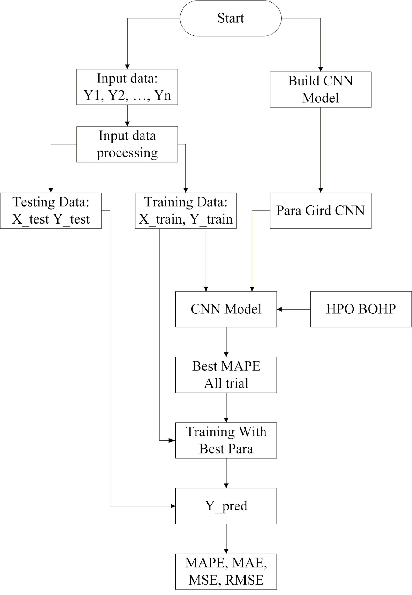
Figure 1. Hyperparameter Optimization and CNN Model Training Process for Electric Load Forecasting
(4) Training with the optimal hyperparameters. Once the optimization process is completed, the configuration that achieves the lowest mean validation MAPE is selected as the best hyperparameter set. A final CNN model is then trained from scratch on the entire training set using this configuration, with the Adam optimizer (learning rate 0.001) and an EarlyStopping callback (patience = 20) to prevent overfitting and unnecessary computation.
(5) Model evaluation and forecasting. The optimized CNN model is evaluated on the held-out test set using standard regression metrics, including MAE, MSE, RMSE, and MAPE. The total runtime for hyperparameter optimization is also recorded to assess computational efficiency. The trained model is then used to generate short-term load forecasts for future time steps. This systematic workflow—from data preprocessing and model construction to BO-TPE-HB optimization and final evaluation—provides a reproducible and scalable framework for CNN-based STLF in real-world power system applications.
- Evaluation Method
The evaluation procedure in this study is designed to identify the optimal hyperparameter configuration for the CNN-based short-term load forecasting model using the BO-TPE-HB algorithm, while ensuring a fair and leakage-free assessment of predictive performance. All experiments are conducted under the same computational environment, with a fixed random seed (RNG_SEED = 42) for both NumPy and TensorFlow, to ensure reproducibility.
First, the historical half-hourly load time series is split chronologically into a training set and a test set, preserving temporal order (approximately 80% of the data for training and 20% for testing). The test set is kept completely untouched during hyperparameter optimization. For the training portion only, we apply a 3-fold time-series cross-validation scheme using TimeSeriesSplit to respect the temporal structure and prevent data leakage between the training and validation data. In each fold, the model is trained on earlier observations and validated on later observations.
Within each BO-TPE-HB trial, the CNN model is trained with a specific hyperparameter configuration sampled from the predefined search space. The search space includes the number of convolutional filters in each layer  , the loss function (
 (
( ), and the maximum number of training epochs (
 ), which serves as the resource variable for Hyperband. The 1D-CNN architecture follows the design described in Section 2.1, which consists of four Conv1D layers with ReLU activation and “same” padding, followed by a Flatten layer, a Dense(64, ReLU) layer, a Dropout (0.2) layer, and a linear Dense (1) output layer.
The model is trained using the Adam optimizer with a learning rate of 0.001, and an EarlyStopping callback with a patience of 20 epochs is employed to terminate training when the validation loss no longer improves. In addition, the BO-TPE-HB pruning callback computes the Mean Absolute Percentage Error (MAPE) on the validation fold after each epoch. It reports the intermediate results to the Hyperband scheduler. This allows underperforming trials to be pruned early, significantly reducing computational costs while maintaining robust evaluation quality. For each trial, the model’s performance is evaluated on all three train–validation splits, and the average validation MAPE across the three folds is used as the objective value for the BO-TPE-HB optimization.
After completing all 100 trials, the configuration that achieves the lowest mean validation MAPE is selected as the best hyperparameter set. Using this configuration, the final CNN model is retrained from scratch on the entire training set with EarlyStopping, and then evaluated on the held-out test set. The following performance metrics are computed to assess forecasting accuracy:
In implementation, a small constant, epsilon, is added to the denominator when computing MAPE to avoid division by zero. However, the load series in our dataset does not contain zero values. In addition to these error metrics, we also record the total hyperparameter optimization runtime of BO-TPE-HB to evaluate its computational efficiency and compare the trade-off between accuracy and runtime with other tuning methods.
- RESULT AND DISCUSSION
- Data
In this study, we utilized real electricity load data from two Australian states, New South Wales (NSW) and Victoria (VIC), to evaluate the performance of the forecasting model under different regional conditions. The data, provided by the Australian Energy Market Operator (AEMO), consist of total electricity demand values (measured in MW) recorded every 30 minutes from May 1, 2009, to May 31, 2014. Each dataset contains approximately 43,000 half-hourly records, corresponding to about five consecutive years of data for each state.
The time-series load data were flattened during preprocessing into a one-dimensional array to facilitate the generation of training samples. Each input sample was constructed using a sliding window approach: the model takes the previous 48 consecutive load values (equivalent to 24 hours) as input and predicts the load for the next 30-minute step. This window structure enables the model to capture daily consumption cycles and short-term temporal dependencies effectively.
For each region, the dataset was divided chronologically into 80% for training and 20% for testing, preserving the temporal order (with shuffling disabled). The training and testing datasets were then reshaped into three-dimensional arrays (samples, timesteps, features) to match the input requirements of deep learning models such as CNN or LSTM. A total of 1,680 samples were used in each experiment, including 1,344 training samples and 336 testing samples, corresponding to the most recent segment of the study period.
Before training, the data had already undergone quality verification and integrity checks by AEMO, so no additional handling of missing values or outliers was required. Furthermore, descriptive statistics, including mean, standard deviation, minimum, and maximum values, were computed to provide an overview of the load series characteristics. The load series exhibit clear daily and weekly patterns, as well as seasonal variations, particularly during the summer and winter months. NSW and VIC exhibit significant peak-hour fluctuations due to high urban population density and increased air conditioning demand during hot weather conditions.
This statistical analysis and data-structure design form a crucial foundation for selecting an appropriate deep learning model architecture, ensuring the model’s ability to capture both short-term temporal features and longer-term seasonal trends in the short-term load forecasting task.
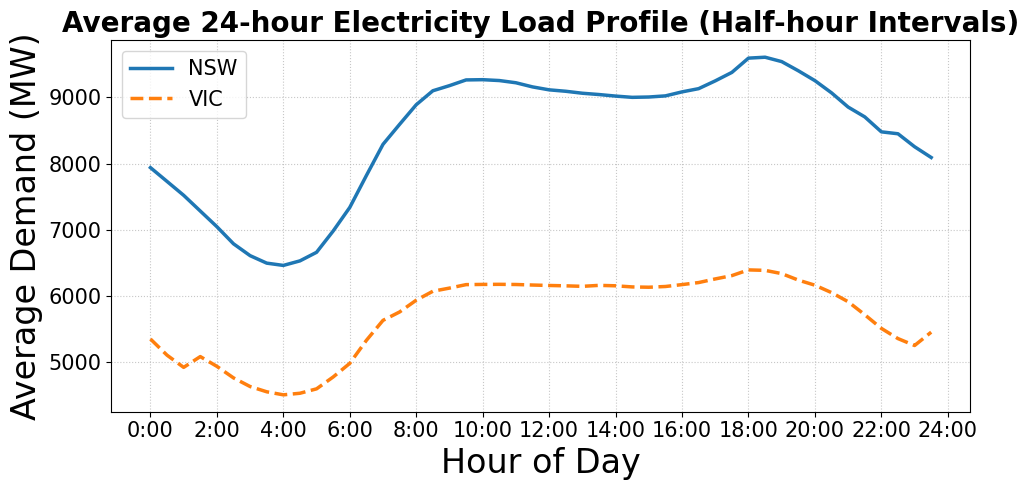
Figure 2 presents the average 24-hour electricity load profiles of New South Wales (NSW) and Victoria (VIC) based on half-hourly data recorded from 2009 to 2014. The Figure 2 shows a clear day–night consumption cycle in both regions. The load reaches its lowest level during the early morning hours (around 4:00–5:00). It rises sharply to a pronounced evening peak between 18:00 and 20:00. The average demand in NSW is consistently higher than in VIC, reflecting its larger population and greater industrial activity. The similar shapes of the two curves indicate a strong correlation in energy consumption behavior and temporal usage patterns between the two states.
Figure 2. Average 24-hour electricity load profiles of New South Wales (NSW) and Victoria (VIC) based on half-hourly data from 2009 to 2014
- Main Results
Figure 3 to Figure 6 present a comparative analysis between the actual load values (y_test) and the forecasting results of the CNN model under four different hyperparameter optimization strategies: the baseline CNN model without optimization, CNN optimized using Random Search, CNN optimized using Bayesian Optimization, and CNN optimized using the Bayesian Optimization with Hyperband (BO-TPE-HB) approach.
In Figure 3, the baseline CNN model demonstrates a reasonable ability to capture the overall load patterns, with the predicted curve closely following the actual data during most peak and off-peak cycles. However, noticeable deviations remain at several peak points, indicating that the model’s performance is limited without hyperparameter optimization. Figure 4 shows that the CNN model optimized using Random Search achieves improved alignment with the actual load data in some regions, particularly around troughs and periods with moderate fluctuations. Nevertheless, due to the unguided nature of the search process, Random Search does not systematically explore promising regions of hyperparameters. Interestingly, on the NSW dataset, Random Search even underperforms the untuned baseline in terms of several error metrics (Table 1). This suggests that purely random exploration can occasionally select poor hyperparameter combinations, resulting in model performance that is inferior to that of a sensible default configuration.
In Figure 5, the CNN model tuned with Bayesian Optimization exhibits significantly enhanced performance, as the predicted curve almost overlaps with the actual load throughout the entire time series. The reduction in errors at both peaks and troughs demonstrates that the Bayesian approach effectively guides the search toward promising hyperparameter regions, enabling the model to better capture the intrinsic characteristics of the time series. Finally, Figure 6 illustrates the superior performance of the CNN model optimized with the BO-TPE-HB approach. The predicted load curve nearly coincides with the actual data across all regions, including extreme points and transition phases. By combining the advantages of Bayesian Optimization (guided search) and Hyperband (early stopping of poor configurations), BO-TPE-HB efficiently identifies optimal hyperparameter settings while reducing computational cost.
In conclusion, the results in Figure 3 to Figure 6 highlight the crucial role of hyperparameter optimization in improving CNN forecasting performance. The baseline model captures general trends but exhibits considerable errors. Random Search offers moderate improvement but remains suboptimal. Bayesian Optimization achieves higher accuracy, and BO-TPE-HB delivers the best performance with the most accurate and stable predictions. These findings confirm BO-TPE-HB as the most effective strategy, offering a powerful solution for precise and practical short-term load forecasting in real-world power system applications.
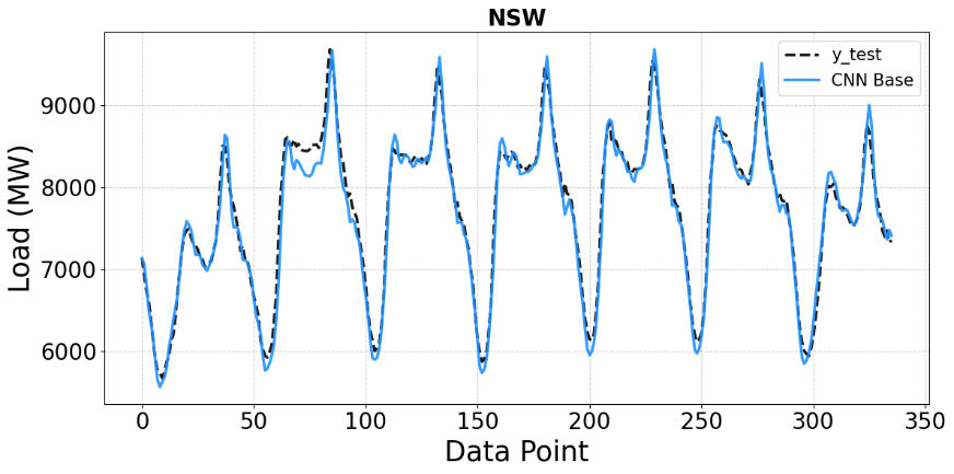
Figure 3. Comparison of CNN Base predictions with ground truth on the NSW test set (MW)
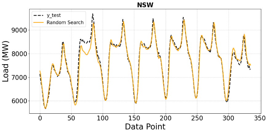
Figure 4. Comparison of Random Search predictions with ground truth on the NSW test set (MW)
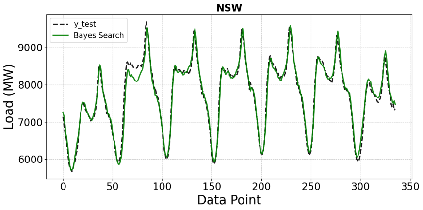
Figure 5. Comparison of Bayes Search predictions with ground truth on the NSW test set (MW)
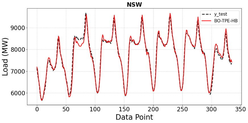
Figure 6. Comparison of BO-TPE-HB predictions with ground truth on the NSW test set (MW)
Figures 7 to Figure 10 present analogous comparisons for the VIC dataset under the same four hyperparameter optimization strategies. In Figure 7, the baseline CNN model captures the general trend and periodic patterns of the VIC load profile, as the predicted curve closely follows the actual data across most data points. However, noticeable deviations remain around peak load values, again indicating limited predictive performance without proper tuning. Figure 8 shows the forecasting results of the CNN model optimized using Random Search. Compared to the baseline, the prediction curve aligns better with the actual load in some low-load and transitional regions; however, residual discrepancies remain at several extreme points, confirming that Random Search improves performance only moderately and does not achieve complete optimization.
In Figure 9, the CNN model optimized using Bayesian Optimization achieves substantially improved accuracy: the predicted curve almost perfectly overlaps with the actual load curve throughout much of the time series, with visibly more minor errors at both peaks and troughs. This confirms that Bayesian Optimization can effectively exploit information from past evaluations to refine the hyperparameter configuration.
Finally, Figure 10 demonstrates the performance of the BO-TPE-HB–optimized CNN on the VIC dataset. The prediction curve closely follows the actual load across most regions, including sharp transitions. For VIC, BO-TPE-HB achieves the lowest MAE and MAPE among all methods, indicating more robust average performance; however, its MSE and RMSE are slightly higher than those of pure Bayesian Optimization (Table 1). This nuance suggests that BO-TPE-HB may incur a few larger individual errors (which inflate MSE/RMSE) even while minimizing the average percentage error. In other words, BO-TPE-HB improves overall robustness, whereas Bayesian Optimization performs marginally better on the worst-case errors in VIC.
Figure 11 and Figure 12 compare the total execution time required by the different hyperparameter optimization strategies for CNN models on the NSW and VIC datasets, respectively. In Figure 11, the baseline CNN model, without optimization, achieves the shortest execution time (approximately 21.34 seconds) because no hyperparameter tuning is performed. Random Search requires a substantially longer runtime (11,725.46 seconds) because it evaluates many configurations with the full training budget in an unguided manner. Bayesian Optimization delivers strong predictive performance but at the highest computational cost (13,008.90 seconds), since each of its 100 trials is trained with the maximum resource budget. In contrast, BO-TPE-HB completes in 10,415.05 seconds, significantly reducing tuning time compared with pure Bayesian Optimization while maintaining superior or comparable forecasting performance.
A similar pattern appears in Figure 12 for the VIC dataset. The baseline CNN again has the shortest runtime (21.80 seconds). Random Search takes 6,769.00 seconds, reflecting its random and inefficient search behavior. Bayesian Optimization requires the most extended runtime (13,827.11 seconds), while BO-TPE-HB completes in only 5,893.94 seconds. This time reduction is primarily due to Hyperband’s multi-fidelity pruning. Random Search and pure Bayesian Optimization effectively train all trials at or near the whole epoch budget. In contrast, BO-TPE-HB terminates many underperforming configurations early, thereby reducing the total number of epochs actually executed.
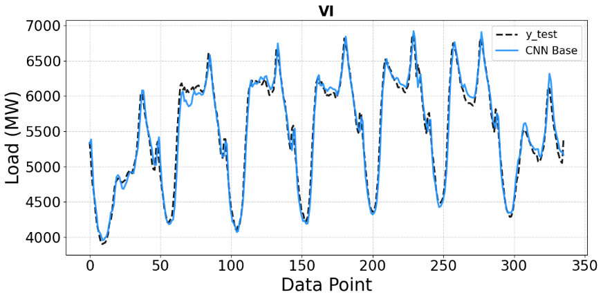
Figure 7. Comparison of CNN Base predictions with ground truth on the test set (MW)
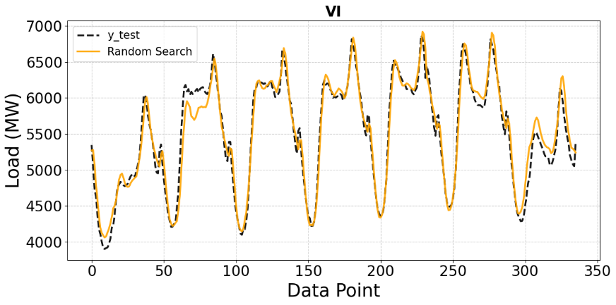
Figure 8. Comparison of Random Search predictions with ground truth on the VI test set (MW)
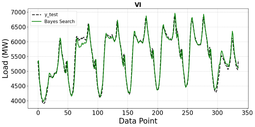
Figure 9. Comparison of Bayes Search predictions with ground truth on the VI test set (MW)
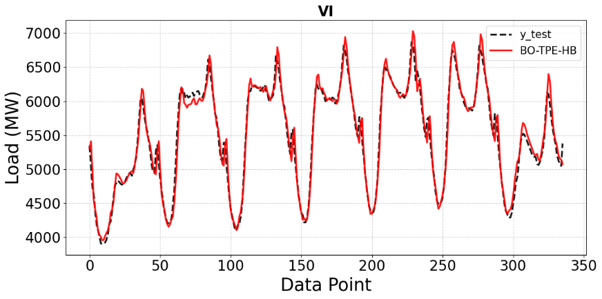
Figure 10. Comparison of BO-TPE-HB predictions with ground truth on the VI test set (MW)
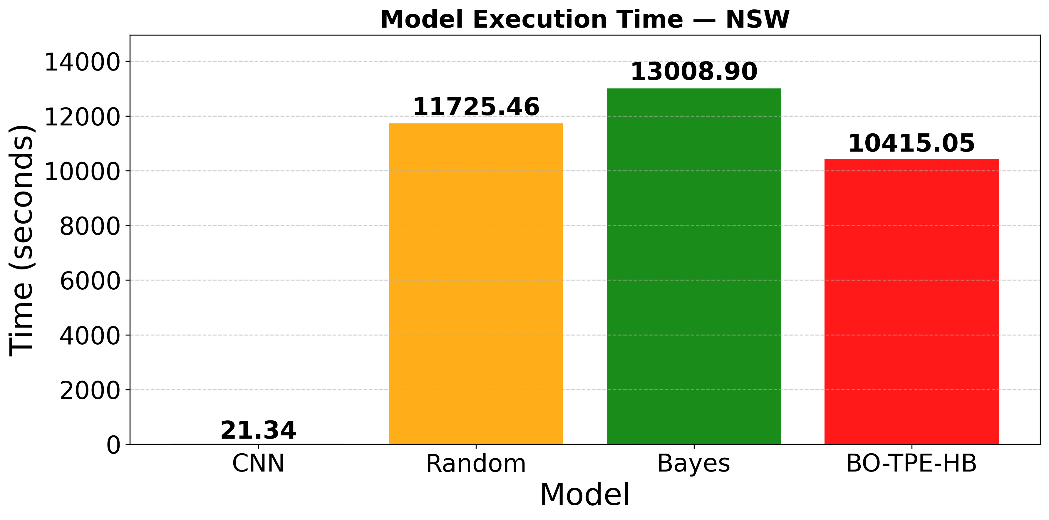
Figure 11. Comparison of total hyperparameter tuning time for different optimization methods on the NSW dataset
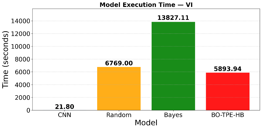
Figure 12. Comparison of total hyperparameter tuning time for different optimization methods on the VI dataset
Table 1 presents the performance comparison of the CNN model under the four hyperparameter optimization strategies — baseline CNN (no optimization), Random Search, Bayesian Optimization, and BO-TPE-HB — evaluated on the NSW and VIC datasets. Table 1 summarizes key forecasting metrics, including MAE, MSE, RMSE, MAPE, and total execution time, thereby providing a comprehensive view of the trade-off between prediction accuracy and computational cost. For the NSW dataset, the baseline CNN achieves an MAE of 112.7331, an RMSE of 147.1660, and an MAPE of 1.4651%, with the shortest runtime (21.34 s), as it does not involve hyperparameter tuning. Random Search performs worse overall, with the highest errors (MAE = 123.8821, RMSE = 177.6061, MAPE = 1.5802%) and a substantial runtime (11,725.46 s), highlighting the inefficiency and potential risk of unguided random exploration. Bayesian Optimization improves prediction accuracy (MAE = 114.1438, RMSE = 152.1085, MAPE = 1.4711%) but at the cost of the most extended runtime (13,008.90 s) due to its fully budgeted model-based search. The BO-TPE-HB approach demonstrates the best overall trade-off, achieving the lowest errors (MAE = 105.9752, RMSE = 143.7076, MAPE = 1.3503%) while also significantly reducing runtime relative to Bayesian Optimization (10,415.05 s).
A similar trend is observed for the VIC dataset. The baseline CNN shows moderate accuracy (MAE = 94.2967, RMSE = 121.2021, MAPE = 1.7228%) with minimal runtime (21.80 s). Random Search again yields the weakest results (MAE = 122.3198, RMSE = 156.5887, MAPE = 2.2511%) and a relatively high runtime (6,769.00 s). Bayesian Optimization enhances predictive performance with lower errors (MAE = 92.6490, RMSE = 123.6352, MAPE = 1.6959%) but requires the highest computational cost (13,827.11 s). BO-TPE-HB provides the most favorable balance, achieving the lowest MAE (89.1329) and a reduced MAPE (1.6146%), while cutting the execution time to 5,893.94 s, which is markedly lower than that of Bayesian Optimization. As noted above, its slightly higher MSE and RMSE compared with Bayesian Optimization in VIC reflect a small number of larger individual errors rather than systematically worse performance.
In summary, Table 1 and Figure 3 to Figure 12 collectively demonstrate that hyperparameter optimization has a significant impact on both forecasting accuracy and computational efficiency. The baseline CNN is computationally efficient but less accurate. Random Search is both less precise and less efficient. Bayesian Optimization achieves high accuracy but at a considerable runtime. In contrast, BO-TPE-HB consistently delivers the best overall combination of accuracy and tuning time.
Table 1. Performance comparison of CNN models with different hyperparameter optimization strategies on NSW and VI datasets
ERROR | CNN | RANDOM | BAYES | BO-TPE-HB | Place |
MAE | 112.7331 | 123.8821 | 114.1438 | 105.9752 | NSW |
MSE | 21657.82 | 31543.94 | 23137.01 | 20651.88 | NSW |
RMSE | 147.166 | 177.6061 | 152.1085 | 143.7076 | NSW |
MAPE | 1.465077 | 1.580174 | 1.471074 | 1.350253 | NSW |
TIME | 21.34321 | 11725.46 | 13008.9 | 10415.05 | NSW |
MAE | 94.29674 | 122.3198 | 92.64898 | 89.13291 | VI |
MSE | 14689.95 | 24520.02 | 15285.66 | 15438.14 | VI |
RMSE | 121.2021 | 156.5887 | 123.6352 | 124.2503 | VI |
MAPE | 1.722847 | 2.251064 | 1.695903 | 1.614633 | VI |
TIME | 21.80284 | 6768.999 | 13827.11 | 5893.937 | VI |
- Discussion
The experimental results clearly demonstrate that hyperparameter optimization plays a crucial role in enhancing both predictive accuracy and computational efficiency for CNN-based short-term load forecasting (STLF) models. Across both datasets—New South Wales (NSW) and Victoria (VIC)—the proposed BO-TPE-HB framework consistently outperforms the baseline CNN, Random Search, and standard Bayesian Optimization when the overall trade-off between accuracy and runtime is considered. For NSW, the BO–TPE–HB–optimized CNN achieves the lowest MAE (105.98 MW) and MAPE (1.35%), while reducing total tuning time by approximately 20% compared to pure Bayesian Optimization. For VIC, BO-TPE-HB achieves the lowest MAE (89.13 MW) and a competitive MAPE (1.61%), while substantially reducing the tuning time compared to plain Bayesian Optimization. By contrast, Random Search occasionally underperforms even the untuned baseline, confirming that unguided random exploration can select suboptimal hyperparameters that degrade performance below a reasonable default configuration.
In terms of forecasting accuracy, the obtained MAPE values (approximately 1.35% for NSW and 1.61% for VIC) place the proposed CNN with BO-TPE-HB hyperparameter tuning among the more accurate STLF approaches reported in recent work. Previous CNN- and LSTM-based models for regional short-term load forecasting typically report MAPE in the range of about 1.8–3% on hourly or half-hourly datasets under comparable settings [30]–[38]. Although a strict one-to-one comparison is not possible due to differences in datasets, feature sets, and experimental protocols, these results indicate that a relatively compact univariate 1D-CNN, when carefully tuned using BO-TPE-HB, can achieve error levels that are competitive with or better than those obtained by more complex architectures in the literature.
The performance gains of BO-TPE-HB can be traced to the complementary roles of its two components. The Tree-structured Parzen Estimator (TPE) probabilistically models promising regions of the hyperparameter space based on prior evaluations, thereby guiding the search toward configurations likely to yield lower errors. Hyperband’s successive halving (SH) strategy, in turn, allocates resources in a multi-fidelity manner and efficiently prunes underperforming configurations early. As a result, BO-TPE-HB avoids the inefficiency of Random Search, which expends resources on many poor configurations, and mitigates the high computational cost of exhaustive Bayesian exploration, which trains every configuration with the full budget. The nuanced behavior observed for the VIC dataset—where BO-TPE-HB slightly increases MSE/RMSE but reduces MAE/MAPE relative to pure Bayesian Optimization—suggests that the hybrid method may occasionally incur a few larger individual errors (which impact MSE/RMSE), even while producing more robust average performance. This highlights the importance of evaluating multiple error metrics when comparing forecasting methods, rather than relying on a single indicator.
From a practical perspective, these findings suggest that the proposed BO-TPE-HB framework can be deployed as a tuning layer on top of existing CNN-based STLF tools without imposing prohibitive computational overhead. The reduction in hyperparameter-optimization runtime relative to plain Bayesian Optimization keeps the overall computational effort manageable. At the same time, the achieved MAPE values of approximately 1–2% on both NSW and VIC are sufficiently low for many operational tasks, such as short-term scheduling, reserve planning, and market bidding. Thus, the framework offers a reproducible and automated way to maintain well-tuned CNN forecasting models as new load data become available, avoiding ad-hoc manual tuning and costly exhaustive search, and providing a balanced solution between accuracy and computational cost for real-world power system applications.
This work also has several strengths and limitations. One strength is the demonstration of consistent improvements across two different regions (NSW and VIC), indicating that the BO-TPE-HB framework is robust to variations in load magnitude, seasonal variability, and consumer behavior. Another strength is the explicit consideration of computational cost. By recording the total runtime of hyperparameter optimization, the study demonstrates that BO-TPE-HB provides the best overall method when both accuracy and efficiency are considered. For pure speed, the baseline CNN is obviously the fastest, and for individual metrics such as RMSE on the VIC dataset, pure Bayesian Optimization can be marginally better. However, BO-TPE-HB delivers the most balanced solution, substantially improving accuracy over the baseline and Random Search while maintaining a reasonable tuning time.
On the limitation side, the study does not quantify statistical uncertainty in the reported metrics. Due to computational constraints, each method is run once, and single-run point estimates are reported without confidence intervals or formal hypothesis tests. A more rigorous analysis would involve multiple independent runs with different random seeds and statistical tests (e.g., paired tests on error distributions) to verify the significance and robustness of the observed improvements. In addition, no explicit ablation study is conducted to separate the contributions of TPE (Bayesian search) and Hyperband (multi-fidelity pruning). As a consequence, the study cannot precisely quantify the extent to which the performance gain is attributed to guided search versus resource-efficient early stopping. Future work could compare BO-TPE alone, Hyperband alone, and their combination under identical budgets to better understand their individual and joint effects. Finally, the present study focuses on univariate forecasting using only historical load. Incorporating exogenous variables, such as weather or calendar features, and extending the framework to multivariate settings remain essential directions for further research.
Despite these limitations, the evidence indicates that combining probabilistic model-based optimization with resource-aware early stopping yields a practical and effective framework for CNN-based STLF under realistic computational budgets. The proposed BO-TPE-HB approach provides a strong basis for more advanced hybrid or multiscale forecasting models and for future work on uncertainty quantification and ablation-based analysis of hyperparameter optimization strategies.
- CONCLUSIONS
This paper proposed a CNN-based short-term load forecasting (STLF) framework in which the key hyperparameters of a univariate one-dimensional convolutional neural network (1D-CNN) are tuned using a hybrid Bayesian Optimization–Hyperband strategy (BO-TPE-HB). The method integrates the Tree-structured Parzen Estimator (TPE) for probabilistic, model-based search with Hyperband’s multi-fidelity resource allocation and early pruning. The framework was evaluated using real half-hourly electricity load data from the Australian Energy Market Operator (AEMO) for New South Wales (NSW) and Victoria (VIC), with a rigorous time-series cross-validation protocol employed to prevent information leakage between training and testing periods.
The experimental results confirm that hyperparameter optimization has a decisive impact on the performance of CNN-based STLF models. Across both datasets, BO-TPE-HB consistently achieved lower forecasting errors than the untuned baseline model and Random Search and improved upon pure Bayesian Optimization on most metrics while requiring substantially less tuning time. For NSW, the BO–TPE–HB–optimized CNN achieved an MAE of 105.98 MW and a MAPE of 1.35%. For VIC, it achieved an MAE of 89.13 MW and a MAPE of 1.61%. These MAPE values, around 1–2%, indicate that a relatively compact univariate 1D-CNN, when carefully tuned by BO-TPE-HB, can deliver accuracy levels suitable for many operational tasks, such as short-term scheduling, reserve planning, and market bidding. At the same time, the reduction in total hyperparameter optimization runtime compared with standard Bayesian Optimization shows that the proposed framework offers an attractive balance between forecasting accuracy and computational effort, making it feasible to integrate BO-TPE-HB as an automated tuning layer on top of existing CNN-based forecasting tools.
It is important to note, however, that the improvements are not uniform across all metrics and scenarios. For the VIC dataset, pure Bayesian Optimization achieved slightly lower MSE and RMSE than BO-TPE-HB, suggesting that it may produce marginally smaller worst-case errors. In contrast, BO-TPE-HB yielded more robust average performance (lower MAE and MAPE) at a significantly reduced computational cost. Likewise, the baseline CNN remains the fastest method in absolute terms because it bypasses hyperparameter tuning altogether, but its accuracy is inadequate for applications requiring reliable short-term forecasts. These nuances suggest that BO-TPE-HB should be interpreted as the most balanced approach in this study, offering the best overall trade-off between accuracy and tuning time among the considered strategies, rather than being the best in every isolated aspect.
This work also has several limitations. First, only point estimates from single runs were reported; no confidence intervals or statistical significance tests were conducted due to computational constraints, and the inherent randomness of the optimization process was not fully explored. Second, no ablation analysis was performed to disentangle the individual contributions of the TPE (Bayesian search) component and the Hyperband (multi-fidelity pruning) component; consequently, the exact share of improvement attributable to guided search versus resource-efficient early stopping remains an open question. Third, the experiments were restricted to univariate forecasting using historical load only, without exogenous variables such as weather or calendar features, and focused on a single CNN architecture.
Future work will address these limitations by incorporating uncertainty quantification and robustness analysis over multiple runs, performing ablation studies to isolate the roles of Bayesian search and Hyperband, and extending the framework to multivariate settings with additional explanatory variables. Moreover, applying BO-TPE-HB to other deep learning architectures, such as LSTM, Transformer-based models, or hybrid ensembles, and to other regional or national power systems would further validate the generality and practicality of the proposed hyperparameter optimization strategy for short-term load forecasting.
REFERENCES
- J. Wang, K. Wang, Z. Li, H. Lu, and H. Jiang, “Short-term power load forecasting system based on rough set, information granule and multi-objective optimization,” Appl. Soft Comput., vol. 146, p. 110692, 2023, https://doi.org/10.1016/j.asoc.2023.110692.
- L. Baur, K. Ditschuneit, M. Schambach, C. Kaymakci, T. Wollmann, and A. Sauer, “Jou rna lP,” Energy AI, p. 100358, 2024, https://doi.org/10.1016/j.egyai.2024.100358.
- B. Chen, W. Yang, B. Yan, and K. Zhang, “An advanced airport terminal cooling load forecasting model integrating SSA and CNN-Transformer,” Energy Build., vol. 309, p. 114000, 2024, https://doi.org/10.1016/j.enbuild.2024.114000.
- R. C. Dadhich and P. C. Gupta, “Development of electric load prediction techniques for rajasthan region and suggestive measures for optimum use of energy using multi-objective optimization,” Electr. Power Syst. Res., vol. 214, p. 108837, 2023, https://doi.org/10.1016/j.epsr.2022.108837.
- M. Sharma and P. Kaur, “Fog-based Federated Time Series Forecasting for IoT Data,” J. Netw. Syst. Manag., vol. 32, no. 2, pp. 1–24, 2024, https://doi.org/10.1007/s10922-024-09802-2.
- A. Parizad and C. J. Hatziadoniu, “A Real-Time Multistage False Data Detection Method Based on Deep Learning and Semisupervised Scoring Algorithms,” IEEE Syst. J., vol. 17, no. 2, pp. 1753–1764, 2023, https://doi.org/10.1109/JSYST.2023.3265021.
- C. Wang, G. Wang, Y. Liu, S. Ren, and J. Wang, “Short-term power load forecasting based on parallel decomposition,” Adv. Eng. Informatics, vol. 68, p. 103729, 2025, https://doi.org/10.1016/j.aei.2025.103729.
- N. Shabbir, R. Ahmadiahangar, A. Rosin, M. Jawad, J. Kilter, and J. Martins, “XgBoost based Short-term Electrical Load Forecasting Considering Trends & Periodicity in Historical Data,” 2023 IEEE Int. Conf. Energy Technol. Futur. Grids, no. 856602, pp. 1–6, 2023, https://doi.org/10.1109/ETFG55873.2023.10407926.
- W. Xiong, “Bus load forecasting based on maximum information coefficient and CNN-LSTM model,” 2023 IEEE Int. Conf. Image Process. Comput. Appl., pp. 659–663, 2023, https://doi.org/10.1109/ICIPCA59209.2023.10257944.
- G. Yan, J. Wang, and M. Thwin, “A new Frontier in electric load forecasting: The LSV/MOPA model optimized by modified orca predation algorithm,” Heliyon, vol. 10, no. 2, p. e24183, 2024, https://doi.org/10.1016/j.heliyon.2024.e24183.
- B. Harish, D. Panda, K. R. Konda, and A. Soni, “A Comparative Study of Forecasting Problems on Electrical Load Timeseries Data using Deep Learning Techniques,” Conf. Rec. - Ind. Commer. Power Syst. Tech. Conf., vol. 2023-May, pp. 1–5, 2023, https://doi.org/10.1109/ICPS57144.2023.10142125.
- J. Song, “Optimized XGBoost based sparrow search algorithm for short-term load forecasting,” 2021 IEEE Int. Conf. Comput. Sci. Artif. Intell. Electron. Eng., no. 2, pp. 213–217, 2021, https://doi.org/10.1109/CSAIEE54046.2021.9543453.
- M. Fan, Y. Hu, X. Zhang, H. Yin, Q. Yang and L. Fan, "Short-term Load Forecasting for Distribution Network Using Decomposition with Ensemble prediction," 2019 Chinese Automation Congress (CAC), pp. 152-157, 2019, https://doi.org/10.1109/CAC48633.2019.8997169.
- X. Wang, H. Wang, B. Bhandari, and L. Cheng, AI-Empowered Methods for Smart Energy Consumption: A Review of Load Forecasting, Anomaly Detection and Demand Response, vol. 11, no. 3, 2024. https://doi.org/10.1007/s40684-023-00537-0.
- Y. Luo, C. Gao, D. Wang, Z. Jiang, Y. Lv, and G. Xue, “Predictive model for sag and load on overhead transmission lines based on local deformation of transmission lines,” Electr. Power Syst. Res., vol. 214, 2022, 2023, https://doi.org/10.1016/j.epsr.2022.108811.
- L. Zhang, D. Wu, and X. Luo, “An Error Correction Mid-term Electricity Load Forecasting Model Based on Seasonal Decomposition,” Conf. Proc. - IEEE Int. Conf. Syst. Man Cybern., pp. 2415–2420, 2023, https://doi.org/10.1109/SMC53992.2023.10394531.
- A. Faustine, N. J. Nunes, and L. Pereira, “Efficiency through Simplicity: MLP-based Approach for Net-Load Forecasting with Uncertainty Estimates in Low-Voltage Distribution Networks,” IEEE Trans. Power Syst., vol. 40, no. 1, pp. 46–56, 2024, https://doi.org/10.1109/TPWRS.2024.3400123.
- A. I. Arvanitidis, D. Bargiotas, A. Daskalopulu, D. Kontogiannis, I. P. Panapakidis, and L. H. Tsoukalas, “Clustering Informed MLP Models for Fast and Accurate Short-Term Load Forecasting,” Energies, vol. 15, no. 4, pp. 1–14, 2022, https://doi.org/10.3390/en15041295.
- T. Bashir, H. Wang, M. Tahir, and Y. Zhang, “Wind and solar power forecasting based on hybrid CNN-ABiLSTM, CNN-transformer-MLP models,” Renew. Energy, vol. 239, p. 122055, 2025, https://doi.org/10.1016/j.renene.2024.122055.
- J. H. Kim, B. S. Lee, and C. H. Kim, “A Study on the development of long-term hybrid electrical load forecasting model based on MLP and statistics using massive actual data considering field applications,” Electr. Power Syst. Res., vol. 221, p. 109415, 2023, https://doi.org/10.1016/j.epsr.2023.109415.
- M. Alhussein, K. Aurangzeb, and S. I. Haider, “Hybrid CNN-LSTM Model for Short-Term Individual Household Load Forecasting,” IEEE Access, vol. 8, pp. 180544–180557, 2020, https://doi.org/10.1109/ACCESS.2020.3028281.
- D. Chen, J. Zhang, and S. Jiang, “Forecasting the Short-Term Metro Ridership with Seasonal and Trend Decomposition Using Loess and LSTM Neural Networks,” IEEE Access, vol. 8, pp. 91181–91187, 2020, https://doi.org/10.1109/ACCESS.2020.2995044.
- C. Li, R. Hu, C. Y. Hsu, and Y. Han, “Short-term Power Load Forecasting based on Feature Fusion of Parallel LSTM-CNN,” 2022 IEEE 4th Int. Conf. Power, Intell. Comput. Syst. ICPICS 2022, no. 4, pp. 448–452, 2022, https://doi.org/10.1109/ICPICS55264.2022.9873566.
- Y. Da Jhong, C. S. Chen, B. C. Jhong, C. H. Tsai, and S. Y. Yang, “Optimization of LSTM Parameters for Flash Flood Forecasting Using Genetic Algorithm,” Water Resour. Manag., vol. 38, no. 3, pp. 1141–1164, 2024, https://doi.org/10.1007/s11269-023-03713-8.
- A. Kumar and M. N. Alam, “Bidirectional LSTM Network-Based Short-Term Load Forecasting Method in Smart Grids,” 5th Int. Conf. Energy, Power, Environ. Towar. Flex. Green Energy Technol. ICEPE 2023, pp. 1–6, 2023, https://doi.org/10.1109/ICEPE57949.2023.10201537.
- O. Rubasinghe, X. Zhang, T. K. Chau, T. Fernando, and H. H. C. Iu, “A Novel Sequence to Sequence based CNN-LSTM Model for Long Term Load Forecasting,” Proc. - 2022 IEEE Sustain. Power Energy Conf. iSPEC 2022, pp. 1–5, 2022, https://doi.org/10.1109/iSPEC54162.2022.10033062.
- S. Cantillo-Luna, R. Moreno-Chuquen, and J. A. Lopez Sotelo, “Intra-day Electricity Price Forecasting Based on a Time2Vec-LSTM Neural Network Model,” 2023 IEEE Colomb. Conf. Appl. Comput. Intell. ColCACI 2023 - Proc., pp. 1–6, 2023, https://doi.org/10.1109/ColCACI59285.2023.10225803.
- T. H. Bao Huy, D. N. Vo, K. P. Nguyen, V. Q. Huynh, M. Q. Huynh, and K. H. Truong, “Short-Term Load Forecasting in Power System Using CNN-LSTM Neural Network,” Conf. Proc. - 2023 IEEE Asia Meet. Environ. Electr. Eng. EEE-AM 2023, pp. 1–6, 2023, https://doi.org/10.1109/EEE-AM58328.2023.10395221.
- S. M. H. Rizvi, “Time Series Deep learning for Robust Steady-State Load Parameter Estimation using 1D-CNN,” Arab. J. Sci. Eng., 2021, https://doi.org/10.1007/s13369-021-05782-6.
- Q. Hua et al., “A Short-Term Power Load Forecasting Method Using CNN-GRU with an Attention Mechanism,” Energies, vol. 18, no. 1, pp. 1–17, 2025, https://doi.org/10.3390/en18010106.
- X. Bu, Q. Wu, B. Zhou, and C. Li, “Hybrid short-term load forecasting using CGAN with CNN and semi-supervised regression,” Appl. Energy, vol. 338, p. 120920, 2023, https://doi.org/10.1016/j.apenergy.2023.120920.
- Z. Tian, W. Liu, W. Jiang, and C. Wu, “CNNs-Transformer based day-ahead probabilistic load forecasting for weekends with limited data availability,” Energy, vol. 293, p. 130666, 2024, https://doi.org/10.1016/j.energy.2024.130666.
- X. Chen, M. Yang, Y. Zhang, J. Liu, and S. Yin, “Load Prediction Model of Integrated Energy System Based on CNN-LSTM,” 2023 3rd Int. Conf. Energy Eng. Power Syst. EEPS 2023, pp. 248–251, 2023, https://doi.org/10.1109/EEPS58791.2023.10257124.
- H. Kuang, Q. Guo, S. Li, and H. Zhong, “Short-term Power Load Forecasting Method in Rural Areas Based on CNN-LSTM,” Proc. 2021 IEEE 4th Int. Electr. Energy Conf. CIEEC 2021, pp. 7–11, 2021, https://doi.org/10.1109/CIEEC50170.2021.9510777.
- Ş. Özdemir, Y. Demir, and Ö. Yildirim, “The Effect of Input Length on Prediction Accuracy in Short-Term Multi-Step Electricity Load Forecasting: A CNN-LSTM Approach,” IEEE Access, no. February, 2025, https://doi.org/10.1109/ACCESS.2025.3540636.
- Y. K. Ahranjani, M. Beiraghi, and R. Ghanizadeh, “Short time load forecasting for Urmia city using the novel CNN-LTSM deep learning structure,” Electr. Eng., 2024, https://doi.org/10.1007/s00202-024-02361-4.
- R. Liu, J. Shi, G. Sun, S. Lin, and F. Li, “A Short-term net load hybrid forecasting method based on VW-KA and QR-CNN-GRU,” Electr. Power Syst. Res., vol. 232, p. 110384, 2024, https://doi.org/10.1016/j.epsr.2024.110384.
- H. Xu, F. Hu, X. Liang, G. Zhao, and M. Abugunmi, “A framework for electricity load forecasting based on attention mechanism time series depthwise separable convolutional neural network,” Energy, vol. 299, no. October 2023, p. 131258, 2024, https://doi.org/10.1016/j.energy.2024.131258.
- B. Bischl et al., “Hyperparameter optimization: Foundations, algorithms, best practices, and open challenges,” Wiley Interdiscip. Rev. Data Min. Knowl. Discov., vol. 13, no. 2, pp. 1–43, 2023, https://doi.org/10.1002/widm.1484.
- I. A. Ibrahim and M. J. Hossain, “Short-term multivariate time series load data forecasting at low-voltage level using optimised deep-ensemble learning-based models,” Energy Convers. Manag., vol. 296, p. 117663, 2023, https://doi.org/10.1016/j.enconman.2023.117663.
- P. S. Pravin, J. Z. M. Tan, K. S. Yap, and Z. Wu, “Hyperparameter optimization strategies for machine learning-based stochastic energy efficient scheduling in cyber-physical production systems,” Digit. Chem. Eng., vol. 4, p. 100047, 2022, https://doi.org/10.1016/j.dche.2022.100047.
- S. Atef and A. B. Eltawil, “Assessment of stacked unidirectional and bidirectional long short-term memory networks for electricity load forecasting,” Electr. Power Syst. Res., vol. 187, p. 106489, 2020, https://doi.org/10.1016/j.epsr.2020.106489.
- A. A. M. Warad, K. Wassif, and N. R. Darwish, “An ensemble learning model for forecasting water-pipe leakage,” Sci. Rep., vol. 14, no. 1, pp. 1–17, 2024, https://doi.org/10.1038/s41598-024-60840-x.
- [Z. Sheng, H. Wang, G. Chen, B. Zhou, and J. Sun, “Convolutional residual network to short-term load forecasting,” Appl. Intell., vol. 51, no. 4, pp. 2485–2499, 2021, https://doi.org/10.1007/s10489-020-01932-9.
- M. Vijay and M. Saravanan, “Solar Irradiance Forecasting using Bayesian Optimization based Machine Learning Algorithm to Determine the Optimal Size of a Residential PV System,” Int. Conf. Sustain. Comput. Data Commun. Syst. ICSCDS 2022 - Proc., pp. 744–749, 2022, https://doi.org/10.1109/ICSCDS53736.2022.9761011.
- N. B. Vanting, Z. Ma, and B. N. Jørgensen, “A scoping review of deep neural networks for electric load forecasting,” Energy Informatics, vol. 4, 2021, https://doi.org/10.1186/s42162-021-00148-6.
- R. Panigrahi, N. R. Patne, B. V. Surya Vardhan, and M. Khedkar, “Short-term load analysis and forecasting using stochastic approach considering pandemic effects,” Electr. Eng., vol. 106, no. 3, pp. 3097–3108, 2024, https://doi.org/10.1007/s00202-023-02135-4.
- J. Cardo-Miota, R. Trivedi, S. Patra, S. Khadem, and M. Bahloul, “Data-driven approach for day-ahead System Non-Synchronous Penetration forecasting: A comprehensive framework, model development and analysis,” Appl. Energy, vol. 362, 2024, https://doi.org/10.1016/j.apenergy.2024.123006.
- A. D. Manchalwar, N. R. Patne, B. V. S. Vardhan, and M. Khedkar, “Peer-to-peer energy trading in a distribution network considering the impact of short-term load forecasting,” Electr. Eng., vol. 105, no. 4, pp. 2069–2081, 2023, https://doi.org/10.1007/s00202-023-01793-8.
- S. Hanifi, A. Cammarono, and H. Zare-Behtash, “Advanced hyperparameter optimization of deep learning models for wind power prediction,” Renew. Energy, vol. 221, p. 119700, 2024, https://doi.org/10.1016/j.renene.2023.119700.
- M. Madhiarasan, “Bayesian optimisation algorithm based optimised deep bidirectional long short term memory for global horizontal irradiance prediction in long-term horizon,” Front. Energy Res., vol. 13, pp. 1–15, 2025, https://doi.org/10.3389/fenrg.2025.1499751.
- T. N. Tran and T. A. Nguyen, “Hyperparameter Optimization for Deep Learning Modeling in Short-Term Load Forecasting,” Int. J. Electr. Comput. Eng. Syst., vol. 16, no. 6, pp. 443–450, 2025, https://doi.org/10.32985/ijeces.16.6.2.
- T. C. Hakyemez and O. Adar, “Testing the Efficacy of Hyperparameter Optimization Algorithms in Short-Term Load Forecasting,” arXiv preprint arXiv:2410.15047, 2024, https://doi.org/10.48550/arXiv.2410.15047.
- K. V. A. Reddy, S. R. Ambati, Y. S. Rithik Reddy, and A. N. Reddy, “AdaBoost for Parkinson’s Disease Detection using Robust Scaler and SFS from Acoustic Features,” Proc. - 1st Int. Conf. Smart Technol. Commun. Robot. STCR 2021, pp. 1–6, 2021, https://doi.org/10.1109/STCR51658.2021.9588906.
- Q. Shen, L. Mo, G. Liu, J. Zhou, Y. Zhang, and P. Ren, “Short-Term Load Forecasting Based on Multi-Scale Ensemble Deep Learning Neural Network,” IEEE Access, vol. 11, pp. 111963–111975, 2023, https://doi.org/10.1109/ACCESS.2023.3322167.
- K. Zhu, Y. Li, W. Mao, F. Li, and J. Yan, “LSTM enhanced by dual-attention-based encoder-decoder for daily peak load forecasting,” Electr. Power Syst. Res., vol. 208, p. 107860, 2022, https://doi.org/10.1016/j.epsr.2022.107860.
- N. Giamarelos and E. N. Zois, “Boosting short term electric load forecasting of high & medium voltage substations with visibility graphs and graph neural networks,” Sustain. Energy, Grids Networks, vol. 38, p. 101304, 2024, https://doi.org/10.1016/j.segan.2024.101304.
- J. F. Torres, D. Gutiérrez-Avilés, A. Troncoso, and F. Martínez-Álvarez, “Random Hyper-parameter Search-Based Deep Neural Network for Power Consumption Forecasting,” Lect. Notes Comput. Sci. (including Subser. Lect. Notes Artif. Intell. Lect. Notes Bioinformatics), vol. 11506 LNCS, pp. 259–269, 2019, https://doi.org/10.1007/978-3-030-20521-8_22.
- C. Xu and G. Chen, “Interpretable transformer-based model for probabilistic short-term forecasting of residential net load,” Int. J. Electr. Power Energy Syst., vol. 155, p. 109515, 2024, https://doi.org/10.1016/j.ijepes.2023.109515.
- A. Groß, A. Lenders, F. Schwenker, D. A. Braun, and D. Fischer, “Comparison of short-term electrical load forecasting methods for different building types,” Energy Informatics, vol. 4, 2021, https://doi.org/10.1186/s42162-021-00172-6.
- W. G. Buratto, R. N. Muniz, A. Nied, and G. V. Gonzalez, “Seq2Seq-LSTM with Attention for Electricity Load Forecasting in Brazil,” IEEE Access, vol. 12, pp. 1–1, 2024, https://doi.org/10.1109/access.2024.3365812.
- A. Jahani, K. Zare, and L. Mohammad Khanli, “Short-term load forecasting for microgrid energy management system using hybrid SPM-LSTM,” Sustain. Cities Soc., vol. 98, p. 104775, 2023, https://doi.org/10.1016/j.scs.2023.104775.
- F. Widmer, S. Nowak, B. Bowler, P. Huber, and A. Papaemmanouil, “Data-driven comparison of federated learning and model personalization for electric load forecasting,” Energy AI, vol. 14, p. 100253, 2023, https://doi.org/10.1016/j.egyai.2023.100253.
- E. Yang and C. H. Youn, “Temporal Data Pooling With Meta-Initialization for Individual Short-Term Load Forecasting,” IEEE Trans. Smart Grid, vol. 14, no. 4, pp. 3246–3258, 2023, https://doi.org/10.1109/TSG.2022.3225805.
- S. Li, J. Wang, H. Zhang, and Y. Liang, “Short-term load forecasting system based on sliding fuzzy granulation and equilibrium optimizer,” Appl. Intell., vol. 53, no. 19, pp. 21606–21640, 2023, https://doi.org/10.1007/s10489-023-04599-0.
- S. Ryu and Y. Yu, “Quantile-Mixer: A Novel Deep Learning Approach for Probabilistic Short-term Load Forecasting,” IEEE Trans. Smart Grid, vol. 15, no. 2, pp. 2237–2250, 2023, https://doi.org/10.1109/TSG.2023.3290180.
- V. K. Saini, R. Kumar, A. S. Al-Sumaiti, A. Sujil, and E. Heydarian-Forushani, “Learning based short term wind speed forecasting models for smart grid applications: An extensive review and case study,” Electr. Power Syst. Res., vol. 222, p. 109502, 2023, https://doi.org/10.1016/j.epsr.2023.109502.
- R. Kottath, P. Singh, and A. Bhowmick, Swarm-based hybrid optimization algorithms: an exhaustive analysis and its applications to electricity load and price forecasting, vol. 27, no. 19. Springer Berlin Heidelberg, 2023. https://doi.org/10.1007/s00500-023-07928-0.
- R. Chandrasekaran and S. K. Paramasivan, “Advances in Deep Learning Techniques for Short-term Energy Load Forecasting Applications: A Review,” Arch. Comput. Methods Eng., vol. 32, no. 2, pp. 663–692, 2024, https://doi.org/10.1007/s11831-024-10155-x.
- X. Li, H. Guo, L. Xu, and Z. Xing, “Bayesian-Based Hyperparameter Optimization of 1D-CNN for Structural Anomaly Detection,” Sensors, vol. 23, no. 11, 2023, https://doi.org/10.3390/s23115058.
- A. Irankhah, S. R. Saatlou, M. H. Yaghmaee, S. Ershadi-Nasab, and M. Alishahi, “A parallel CNN-BiGRU network for short-term load forecasting in demand-side management,” 2022 12th Int. Conf. Comput. Knowl. Eng. ICCKE 2022, pp. 511–516, 2022, https://doi.org/10.1109/ICCKE57176.2022.9960036.
- A. Neubauer, S. Brandt, and M. Kriegel, “Explainable multi-step heating load forecasting: Using SHAP values and temporal attention mechanisms for enhanced interpretability,” Energy AI, vol. 20, p. 100480, 2025, https://doi.org/10.1016/j.egyai.2025.100480.
AUTHOR BIOGRAPHY

| Trung Dung Nguyen was born in 1976 in Vietnam. He received a Master’s degree in Electrical Engineering from Ho Chi Minh City University of Technology and Education, Vietnam, in 2017. He lectures at the Faculty of Electrical Engineering Technology, Industrial University of Ho Chi Minh City, Ho Chi Minh City, Vietnam. His research focuses on applications of metaheuristic algorithms in power system optimization, optimal control, and model predictive control. Email: nguyentrungdung@iuh.edu.vn |
|
|

| Nguyen Anh Tuan     received a B.Sc. degree from the Industrial University of Ho Chi Minh City, Vietnam 2012, and an M.Sc. degree from the HCMC University of Technology and Education, Vietnam, in 2015. He is a Lecturer with the Faculty of Electrical Engineering Technology at the Industrial University of Ho Chi Minh City, Vietnam. His main research interests include power quality and load forecasting. received a B.Sc. degree from the Industrial University of Ho Chi Minh City, Vietnam 2012, and an M.Sc. degree from the HCMC University of Technology and Education, Vietnam, in 2015. He is a Lecturer with the Faculty of Electrical Engineering Technology at the Industrial University of Ho Chi Minh City, Vietnam. His main research interests include power quality and load forecasting. Email: nguyenanhtuan@iuh.edu.vn |
Trung Dung Nguyen (Hybrid Bayesian–Hyperband Optimization of a One-Dimensional Convolutional Neural Network for Short-Term Load Forecasting)