ISSN: 2685-9572 Buletin Ilmiah Sarjana Teknik Elektro
Vol. 7, No. 4, December 2025, pp. 668-683
Hybrid Stacking of Multilayer Perceptron, Convolutional Neural Network, and Light Gradient Boosting Machine for Short-Term Load Forecasting
Trung Dung Nguyen, Nguyen Anh Tuan
FEET, Industrial University of Ho Chi Minh City, Ho Chi Minh City, Viet Nam
ARTICLE INFORMATION |
| ABSTRACT |
Article History: Received 05 August 2025 Revised 24 September 2025 Accepted 18 October 2025 |
| 
Short-term load forecasting (STLF) is essential for scheduling, dispatch, and demand-side management. Real-world load series exhibit rapid local fluctuations and calendar or exogenous influences that challenge single-model approaches. This study proposes a hybrid stacking framework combining a Multilayer Perceptron (MLP), a 1-D Convolutional Neural Network (CNN), and a Light Gradient Boosting Machine (LightGBM), integrated through a ridge-regression meta-learner. The CNN extracts local temporal patterns from sliding windows of the load series, and the MLP processes tabular features such as lags, rolling statistics, and calendar/holiday indicators. At the same time, LightGBM captures nonlinear interactions in the same feature space. Base learners are trained using a rolling TimeSeriesSplit to avoid temporal leakage, and their out-of-fold predictions are used as inputs for the meta-learner. Early stopping regularizes the neural models. Experimental backtests on Queensland electricity demand data (89,136 half-hourly samples) demonstrate that the stacked model achieves markedly lower forecasting errors, with MAPE ≈ 0.81%, corresponding to a 24% reduction compared to CNN (MAPE ≈ 1.07%) and a 32% reduction compared to MLP (MAPE ≈ 1.19%). Regarding runtime, LightGBM is the fastest (25s) but least accurate, while the stacked model requires longer computation (2488s) yet delivers the most reliable forecasts. Overall, the proposed framework balances accuracy and robustness, and it is modular, reproducible, and extensible to additional exogenous inputs or base learners. |
Keywords: Short-Term Load Forecasting; Hybrid Stacking; LightGBM; Convolutional Neural Network; Multilayer Perceptron; Ridge Regression |
Corresponding Author: Nguyen Anh Tuan,
FEET, Industrial University of Ho Chi Minh City, Ho Chi Minh City, Viet Nam.
Email: nguyenanhtuan@iuh.edu.vn |
This work is licensed under a Creative Commons Attribution-Share Alike 4.0 
|
Document Citation: T. D. Nguyen and T. A. Nguyen, “Hybrid Stacking of Multilayer Perceptron, Convolutional Neural Network, and Light Gradient Boosting Machine for Short-Term Load Forecasting,” Buletin Ilmiah Sarjana Teknik Elektro, vol. 7, no. 4, pp. 668-683, 2025, DOI: 10.12928/biste.v7i4.14410. |
INTRODUCTION
Short-Term Load Forecasting (STLF) is indispensable to reliable and economical power system operation. Accurate forecasts, ranging from a few hours to several days ahead, enable effective scheduling, generation dispatch, and resource allocation. With the rapid growth of electricity demand in metropolitan areas, strongly shaped by daily, weekly, and seasonal patterns, achieving high forecasting accuracy is increasingly critical for utilities and consumers. Traditional forecasting methods, including Moving Average (MA) [1]–[5], Linear Regression [6]l–[9], and classical time-series approaches [10]–[11] such as Auto-Regressive Integrated Moving Average (ARIMA) [12]–[17], have been widely applied for decades. These approaches are simple, interpretable, and computationally efficient. However, their limited ability to capture nonlinear dynamics and complex load fluctuations reduces their effectiveness under rapidly changing demand or strong exogenous influences such as weather and holidays.
The emergence of Machine Learning (ML) and Deep Learning (DL) has significantly advanced STLF research. ML methods such as Support Vector Regression (SVR) [18]–[22], Random Forest (RF) [23]–[27], Categorical Boosting (CatBoost) [28]–[31], Extreme Gradient Boosting (XGBoost) [32]–[36], and boosting algorithms like Gradient Boosting and Light Gradient Boosting Machine (LightGBM) [37]–[41] provide strong nonlinear modeling capabilities and robust generalization. Meanwhile, DL architectures including Multilayer Perceptron (MLP) [42]–[46], Convolutional Neural Network (CNN) [47]–[53], Long Short-Term Memory (LSTM) [54]–[63], and Transformer-based models [64]–[65] have shown remarkable success in automatically extracting features and capturing temporal dependencies. Nevertheless, DL models often require large datasets, are prone to overfitting, and demand high computational resources. In contrast, tree-based models may struggle to represent sequential local patterns inherent in load series.
Hybrid frameworks have been proposed to overcome these limitations. Instead of relying on a single learner, stacking ensembles [66]–[69] integrate complementary models into a unified framework. For example, CNN effectively captures local temporal motifs, MLP processes tabular and exogenous features, and LightGBM provides efficient nonlinear regression. A meta-learner can then learn how to combine these base predictions, balancing their strengths and mitigating weaknesses. This study introduces a hybrid stacking model integrating MLP, CNN, and LightGBM through a Ridge-based meta-learner for STLF. The framework is evaluated on a large-scale real-world dataset and benchmarked against individual base learners. Experimental results show that the stacked model consistently improves accuracy across multiple error metrics (MAE, MSE, RMSE, MAPE), particularly during peak load and holiday periods, while maintaining computational feasibility. The contributions of this work are threefold:
- A novel hybrid stacking framework integrating MLP, CNN, and LightGBM with a Ridge-based meta-learner to enhance STLF accuracy.
- Comprehensive evaluation and comparison of base learners and the proposed stacked model, providing insights into their complementary strengths.
- Empirical validation on a real-world dataset that highlights the trade-off between forecasting accuracy and computational cost, offering practical guidance for ensemble-based forecasting frameworks.
MODEL DESCRIPTION
LightGBM - Light Gradient Boosting Machine
LightGBM (Light Gradient Boosting Machine) is a machine learning algorithm belonging to the Gradient Boosting Decision Tree (GBDT) family, developed by Microsoft, designed to optimize training speed, memory efficiency, and the ability to handle large-scale data. In principle, LightGBM inherits the idea of GBDT by constructing multiple decision trees sequentially, where each new tree is trained to minimize the residual error of the previous model, following the general formula:
| 
| (1) |
Where  represents the model at the mthm^{th} iteration,
  is the newly generated decision tree, and η\eta denotes the learning rate. The fundamental distinction of LightGBM compared to traditional GBDT lies in its leaf-wise growth strategy: instead of expanding trees level-wise, LightGBM selects the leaf with the maximum loss reduction for further splitting, which results in higher accuracy but also a greater risk of overfitting if the number of leaves is not constrained by parameters such as max_depth. In addition, LightGBM employs the histogram-based splitting technique, where feature values are discretized into bins, thereby reducing computational cost, saving memory, and accelerating training. With these mechanisms, LightGBM provides multiple advantages, including fast training speed, efficient handling of large and sparse data, GPU support, and high predictive accuracy; however, the model can overfit if hyperparameters are not properly tuned. Key hyperparameters include num_leaves, max_depth, learning_rate, n_estimators, feature_fraction, bagging_fraction, as well as the regularization terms
  and . Thanks to these properties, LightGBM has been widely applied in domains such as classification, regression, ranking, and large-scale data analysis, such as web logs or clickstream data.
MLP – Multilayer Perceptron
The Multi-Layer Perceptron (MLP) is a subclass of artificial neural networks widely used for classification and regression tasks. As a Deep Neural Network (DNN) family member, MLPs can approximate complex nonlinear relationships, making them suitable for high-dimensional and nonlinear problems. An MLP consists of three main components: an Input layer receiving raw features; Hidden layers extracting hierarchical patterns through weighted linear combinations and nonlinear activation functions.; Output layer: produces the final prediction (a class label for classification or a continuous value for regression).
The learning process of an MLP includes forward propagation and backpropagation. In forward propagation, inputs are transformed layer by layer through linear operations and activation functions. Backpropagation then adjusts the weights and biases using gradients of the loss function to minimize prediction errors.
| 
| (2) |
| 
| (3) |
| 
| (4) |
| 
| (5) |
| 
| (6) |
| 
| (7) |
| 
| (8) |
| 
| (9) |
| 
| (10) |
| 
| (11) |
| 
| (12) |
| 
| (13) |
| 
| (14) |
 : Linear combination between the pre-layer output and weights, plus bias;
  : is the weighted matrix between class-1 and class
  ;
;  : Is the output of class-1 ;
  : Is the bias of the class ;
  : is the output of the second class, which is the result after applying the trigger function
 ;
;  : Is the trigger function;
  : Predicted output value; y: Actual value;
  : The derivative of the loss function L for class output ; m: is the number of samples in the training dataset.; : Predicted output value; y: Actual value; Gradient for calculation via trigger function:;
  : The gradient of the loss function for pure input ; : The gradient of the loss function to the output of the class ; : Weighted matrix in the second class ;
  : Learning rate;
  : the derivative (gradient) of the loss function L by weight ; η: Is the speed of learning ; : Bias of the class, making the model more flexible when learning;
  : The derivative of the loss function L for the bias at the class .
CNNs - Convolutional Neural Network
Convolutional Neural Networks (CNNs) are powerful deep learning models that handle grid-like data structures, including images and one-dimensional sequences. While they were first introduced for computer vision applications such as object recognition, image classification, and face detection, CNNs have also shown strong potential in short-term load forecasting (STLF). A CNN is typically composed of several essential components: convolutional layers that learn local patterns through trainable filters, activation functions that add nonlinearity to improve learning capacity, pooling layers that downsample feature maps to lower complexity, and fully connected layers that combine the extracted information to generate the final output.
For time-series forecasting, one-dimensional CNNs apply convolutional kernels across the temporal axis, enabling the model to identify periodic structures such as daily or seasonal demand fluctuations. Compared with recurrent neural networks, CNNs offer faster training, parallel computation, and robust results even when historical data are relatively limited. Nonetheless, their predictive performance highly depends on carefully chosen hyperparameters, including the number of layers, filter sizes, kernel dimensions, learning rate, batch size, and epochs.
 :is the value at position
  in the feature map;
  lter of size m x n.;
  represents the corresponding region in the input image; x is the input of the activation function, which selects the better value between 0 and x. If x is less than 0, the output will be 0; if x is greater than 0, the output will remain x; The ReLU function enhances the neural network’s ability to learn nonlinear features while reducing the vanishing gradient problem, making the model more efficient during training;
  ) is a small region in the feature map; x: is the input from the previous layer; W: is the weighted matrix, and b is the bias vector.
PROPOSED METHOD
Architectures LightGBM
Light Gradient Boosting Machine (LightGBM) is a tree-based gradient boosting framework designed for efficiency and high predictive accuracy. It applies a histogram-based algorithm and a leaf-wise growth strategy with depth constraints, enabling faster training and reduced memory usage compared to level-wise boosting. LightGBM is selected as one of the base learners for short-term load forecasting in this study. The model is trained on tabular features including lagged load values, rolling mean and standard deviation, and calendar indicators such as hour of day, day of week, and holiday flags. This design allows LightGBM to capture nonlinear dependencies and feature interactions effectively.
The hyperparameter search space included number of leaves (31, 63, 127), learning rate (0.05, 0.1, 0.2), number of boosting rounds (100, 300, 500, 1000), maximum depth (–1, 10, 20), feature fraction (0.7–1.0), bagging fraction (0.7–1.0), bagging frequency (1, 5), and both L1 and L2 regularization terms (0–10). After cross-validation, the final configuration chosen was: number of leaves equal to 63, learning rate equal to 0.1, number of boosting rounds equal to 500, maximum depth equal to –1, feature fraction equal to 0.8, bagging fraction equal to 0.8, bagging frequency equal to 5, L1 regularization equal to 1, and L2 regularization equal to 1. This configuration balanced predictive performance and computational efficiency, making LightGBM a strong complement to CNN and MLP within the proposed stacking framework.
Architectures MLP
The Multilayer Perceptron (MLP) is a deep learning baseline for tabular feature modeling. It consists of three hidden layers with 16, 32, and 64 neurons, each activated by the Rectified Linear Unit function. The final output layer uses a linear activation to predict continuous load values. The search space covered batch sizes (16, 32, 64) and epochs (100–500), with early stopping patience fixed at 10. The optimizer used is Adam with a learning rate of 0.001, and the loss function is mean squared error, with mean absolute error tracked as an additional evaluation metric. After cross-validation, the final configuration chosen was a batch size equal to 32 and a maximum of 500 epochs, with early stopping typically halting training earlier based on validation loss. This design ensured stable convergence and avoided overfitting. The MLP played a complementary role within the hybrid stacking framework, focusing on smooth nonlinear mappings from lagged values and exogenous variables.
Architectures CNN
The Convolutional Neural Network (CNN) captures short-term temporal patterns and local dependencies in load sequences. By applying convolution filters across fixed-length sliding windows of the input series, CNN automatically detects cyclical load fluctuations, abrupt changes, and seasonal peaks. The search space included filter sizes (16, 32, 64), kernel sizes (3, 5), and dropout rates (0.1, 0.2, 0.3). The final architecture used three successive one-dimensional convolutional layers with 16, 32, and 64 filters, each with Rectified Linear Unit activation and kernel size equal to 3. The feature maps were flattened and passed through a dense layer of 32 neurons with Rectified Linear Unit activation, followed by a dropout layer with a rate equal to 0.2, and a single linear output neuron. The model was trained using the Adam optimizer with a learning rate of 0.001, a batch size of 32, a maximum of 500 epochs, and an early stopping patience of 10. This setup allowed CNN to specialize in sequence-based learning, complementing MLP and LightGBM, which focused on tabular features and feature interactions.
Optimization method
The optimization of the hybrid stacking framework followed a multi-stage process. Each base learner (MLP, CNN, LightGBM) was optimized individually using the defined hyperparameter search spaces. For MLP and CNN, the Adam optimizer with a learning rate of 0.001 was used, with mean squared error as the loss function and mean absolute error monitored. Batch size was set to 32, and early stopping with patience 10 was applied, with a maximum of 500 epochs. For LightGBM, the final chosen configuration was number of leaves equal to 63, learning rate equal to 0.1, boosting rounds equal to 500, maximum depth equal to –1, feature fraction equal to 0.8, bagging fraction equal to 0.8, bagging frequency equal to 5, L1 regularization equal to 1, and L2 regularization equal to 1.
A key element of the optimization was the generation of out-of-fold predictions using 5-fold TimeSeriesSplit cross-validation, ensuring that validation sets always followed training sets in chronological order to avoid temporal leakage. These out-of-fold predictions from the base learners were concatenated to form a meta-feature matrix. The meta-learner, Ridge regression, was then trained on this meta-feature matrix. The regularization strength alpha was selected as 0.01 from the candidate set {0.0001, 0.001, 0.01, 0.1, 1.0}. Ridge regression was chosen for its robustness against multicollinearity and ability to produce stable weights. This approach allowed the meta-learner to balance the complementary strengths of CNN, MLP, and LightGBM, improving generalization and reducing overfitting.
Algorithm Flowchart
The overall training and inference workflow of the proposed stacking framework is illustrated in Figure 1. Figure 1 illustrates the complete workflow of the hybrid stacking framework, consisting of two main phases: training and inference.The raw load series is preprocessed in the training phase through normalization and feature engineering, including lagged values, rolling statistics, and calendar attributes.
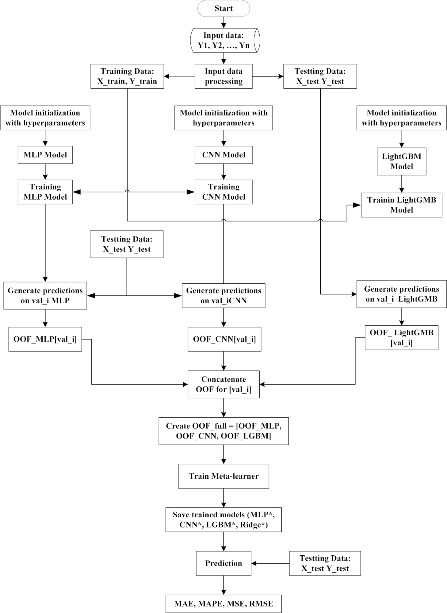
Figure 1. Training and inference workflow of the proposed hybrid stacking framework
The dataset is then divided into training and testing sets. Three base learners—Multilayer Perceptron (MLP), Convolutional Neural Network (CNN), and Light Gradient Boosting Machine (LightGBM)—are initialized with their respective hyperparameters and trained independently. Predictions are generated on validation subsets using a 5-fold TimeSeriesSplit cross-validation strategy, producing out-of-fold predictions (OOF_MLP, OOF_CNN, OOF_LightGBM). These OOF predictions are concatenated into a meta-feature matrix (OOF_full), which is used to train the Ridge regression meta-learner. At the end of this stage, all trained models (MLP, CNN, LightGBM, and Ridge) are saved for later use. In inference, the saved base learners generate predictions on the unseen test set. These predictions are stacked and passed to the Ridge meta-learner, which outputs the final forecasts. The predictive accuracy of the framework is then evaluated using four standard error metrics: Mean Absolute Error (MAE), Mean Absolute Percentage Error (MAPE), Mean Squared Error (MSE), and Root Mean Squared Error (RMSE).
Evaluation Method
This study's evaluation process for short-term load forecasting follows a structured workflow, as shown in Figure 1. The original load series is preprocessed into lag features, rolling statistics, and calendar-based attributes. The processed dataset is then divided chronologically into two subsets: a training set (X_train, Y_train) and a testing set (X_test, Y_test). A 5-fold TimeSeriesSplit cross-validation strategy is applied on the training set to ensure robust training and prevent temporal leakage. In each fold, the three base learners—Multilayer Perceptron (MLP), Convolutional Neural Network (CNN), and Light Gradient Boosting Machine (LightGBM)—are trained independently on the training folds and generate predictions for the validation fold. This produces out-of-fold predictions concatenated to form a meta-feature matrix, which is then used to train the Ridge regression meta-learner. Once the stacking model is finalized, each base learner is retrained on the complete training dataset, and their predictions on the test set are combined through the meta-learner to generate the final forecasts Y_stack.
Forecast accuracy is assessed using four standard error metrics: Mean Absolute Error (MAE), Mean Absolute Percentage Error (MAPE), Mean Squared Error (MSE), and Root Mean Squared Error (RMSE). MAE and MAPE measure the average error magnitude in absolute and relative terms, while MSE and RMSE emphasize larger deviations. This multi-metric approach ensures that model performance is comprehensively evaluated regarding average predictive accuracy and robustness under volatile demand conditions. Although statistical significance tests such as the Diebold–Mariano test are highly valuable for validating forecasting improvements, in this study, we relied on a comprehensive set of error metrics (MAE, MAPE, MSE, RMSE), which already provide a robust and reliable evaluation of model accuracy. Formal significance testing will be conducted in future research to strengthen the conclusions further.
RESULT AND DISCUSSION
Data
The descriptive statistics of the Queensland load data are summarized in Table 1. Table 1 reports the descriptive statistics of the Queensland load series based on 89,136 observations. The mean demand is 5,846 MW, with a median of 5,909 MW and a standard deviation of 839 MW (coefficient of variation ≈ 14.3%), indicating moderate variability. The slightly higher median suggests a mildly left-skewed distribution. The interquartile range spans from Q1 = 5,159 MW to Q3 = 6,438 MW, implying that half of the values fall between 5.2 and 6.4 GW. The minimum is 4,041 MW, while the maximum and peak load reach 8,891 MW, yielding a peak-to-mean ratio of 1.52 and a peak-to-min ratio of 2.20.
Table 1. Descriptive statistics of the load data in Queensland
count | mean | std | min | Peak Load | 25% | 50% | 75% | max | var |
89136 | 5846 | 839 | 4041 | 8891 | 5159 | 5909 | 6438 | 8891 | 703384 |
These values confirm significant intraday fluctuations and the presence of pronounced peaks. The average daily load profile of Queensland is depicted in Figure 2. Figure 2 shows the average daily load curve, highlighting a strong day–night cycle. Demand decreases to a trough of 4.6–4.7 GW in early morning hours (03:00–04:00) and then rises sharply during 05:00–09:00, stabilizing at ~6.2–6.3 GW midday. A second ramp occurs between 16:00 and 19:00, forming the evening peak at ~6.6 GW, roughly 0.8 GW above the plateau. After 20:00, load declines steadily to ~5.6 GW at midnight. This pattern—marked by a pre-dawn valley and an evening peak—indicates that forecasting models must prioritize accuracy during 17:00–20:00 when operational risk is highest. A one-week sample of the load time series is shown in Figure 3. Figure 3 illustrates a 7-day sample of the load series (04–10 Oct 2009), showing regular diurnal patterns. Daily amplitudes reach ~2.1–2.3 GW, with consistent morning up-ramps and evening peaks around 6.6–6.8 GW. Day-to-day variability is relatively small (<≈5%), but weekends exhibit slightly lower midday levels. These observations justify the inclusion of hour-of-day and day-of-week features in the forecasting models.
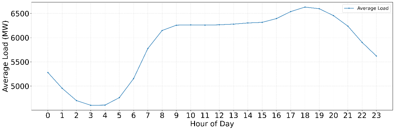
Figure 2. Average Daily Load Profile
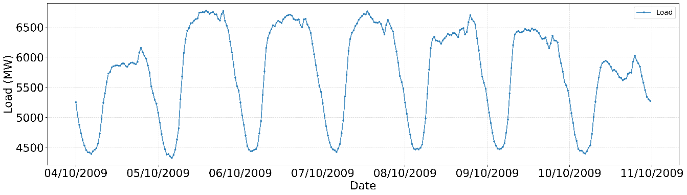
Figure 3. Time Series of Load (7-day sample)
Hyperparameter Grid
The hyperparameter search space for the proposed stacking framework is presented in Table 2. Table 2 summarizes the hyperparameter search space for all models in the stacking framework. For MLP, configurations included three hidden layers (16–64 neurons), ReLU activation, Adam optimizer (learning rate = 0.001), and training up to 500 epochs with early stopping (patience = 10). For CNN, three convolutional layers (filters 16–64), kernel sizes (3, 5), dropout rates (0.1–0.3), and similar optimization settings were considered. LightGBM explored several leaves (31–127), learning rates (0.05–0.2), boosting rounds (100–1000), and various fractions and regularization parameters. The meta-learner Ridge regression tuned α in {0.0001–1.0}.
Through 5-fold TimeSeriesSplit cross-validation, the final configurations selected were:
- MLP: batch size = 32, epochs = 500 (with early stopping), neurons per layer = [16, 32, 64].
- CNN: filters = [16, 32, 64], kernel size = 3, dropout = 0.2, batch size = 32, epochs = 500.
- LightGBM: num_leaves = 63, learning_rate = 0.1, n_estimators = 500, max_depth = –1, feature_fraction = 0.8, bagging_fraction = 0.8, bagging_freq = 5, = 1,
 = 1.
= 1. - Ridge meta-learner: α = 0.01.
This systematic search ensured a fair comparison among models while avoiding overfitting.
Result
Figure 4 to Figure 7 compare the predicted and actual values obtained from LightGBM, MLP, CNN, and the Stacking model. Figure 4 to Figure 7 compare the forecasts of LightGBM, MLP, CNN, and Stacking against the actual load. LightGBM (Figure 4) tracks only the average level (~5,800–6,000 MW) and smooths short-term fluctuations, failing at peaks and troughs. MLP (Figure 5) improves substantially, capturing overall trend and daily cycles, though errors persist at abrupt changes. CNN (Figure 6) aligns closely with the actual load, showing minimal deviations and a strong ability to model recurrent temporal patterns. Stacking (Figure 7) achieves the best performance: its forecasts nearly coincide with actual values, correcting local errors of individual models and providing the most accurate representation of both trend and extremes. These results demonstrate that while LightGBM offers stability, neural models (MLP, CNN) capture temporal dynamics better, and the stacking framework leverages their complementary strengths to achieve superior accuracy.
Figure 8 to Figure 11 present the quantitative evaluation of forecasting performance across all models using MAE, MSE, RMSE, and MAPE. Figure 8 to Figure 11 present the quantitative comparison of forecasting performance across the four models using the evaluation metrics MAE, MSE, RMSE, and MAPE. As shown in Figure 8, the LightGBM model yields a very high mean absolute error (MAE = 571.72), indicating its limitations in closely following the actual data. In contrast, the deep learning models demonstrate substantially better performance, with MLP and CNN achieving MAE values of 79.98 and 60.65, respectively. The Stacking model again shows clear superiority, recording the lowest MAE of 45.74. A similar pattern is observed in Figure 9 for the MSE metric. LightGBM produces a huge error (488,439), whereas MLP and CNN significantly reduce this value to 10,608 and 6,378, respectively. Stacking further improves performance by attaining the lowest MSE of 3,488, confirming its ability to minimize large error magnitudes effectively. The results in Figure 10 reinforce this trend through the RMSE metric. LightGBM records a high RMSE of 698.88, highlighting its weakness in modeling short-term fluctuations. MLP and CNN improve accuracy considerably, with RMSE values of 103.00 and 79.87, respectively. Stacking once again provides the best results, with an RMSE of only 59.06, demonstrating its effectiveness in accurately capturing variations in the load profile.
Finally, Figure 11 evaluates the models using MAPE, which measures relative forecasting accuracy. LightGBM has an MAPE of 10.71%, substantially higher than the neural network–based models. MLP reduces the error to 1.42%, CNN further lowers it to 1.07%, and Stacking achieves the best result at just 0.81%. These findings indicate that the ensemble approach minimizes absolute and squared errors and ensures the highest relative accuracy. The results from Figure 8 to Figure 11 highlight the performance gap among the models. While LightGBM is inadequate for detailed load forecasting, MLP and CNN achieve considerable improvements. Nevertheless, Stacking consistently outperforms all individual models across all evaluation metrics, underscoring the effectiveness of ensemble learning for short-term load forecasting.
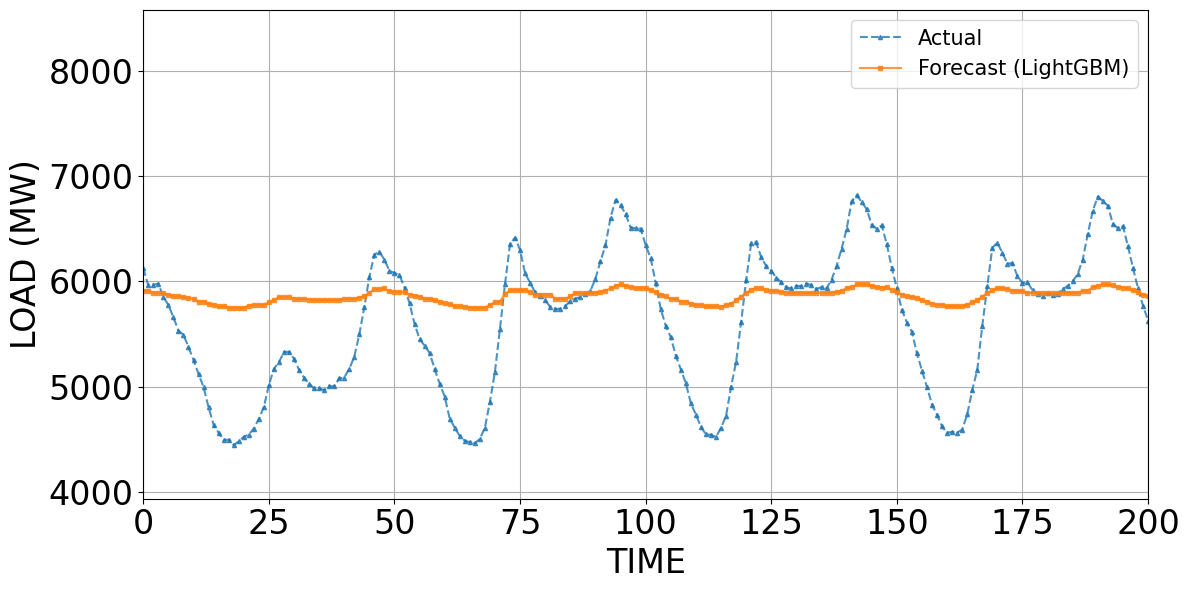
Figure 4. Predicted and actual values using the LightGBM model
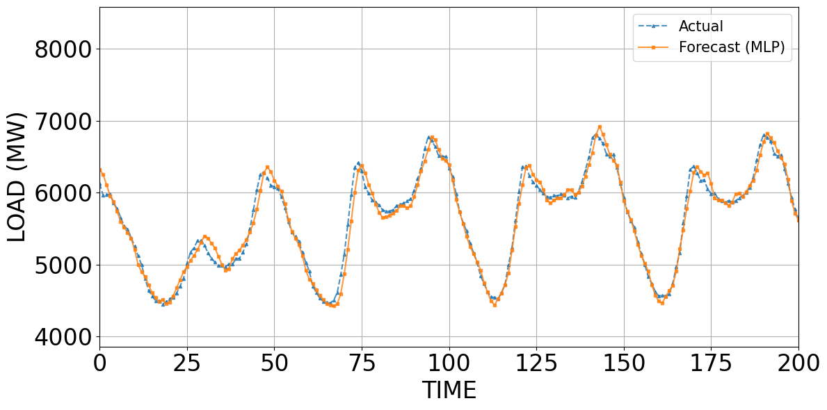
Figure 5. Predicted and actual values using the MLP model
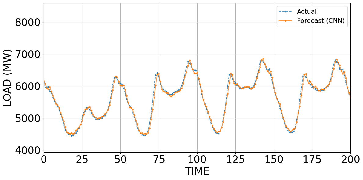
Figure 6. Predicted and actual values using the CNN model
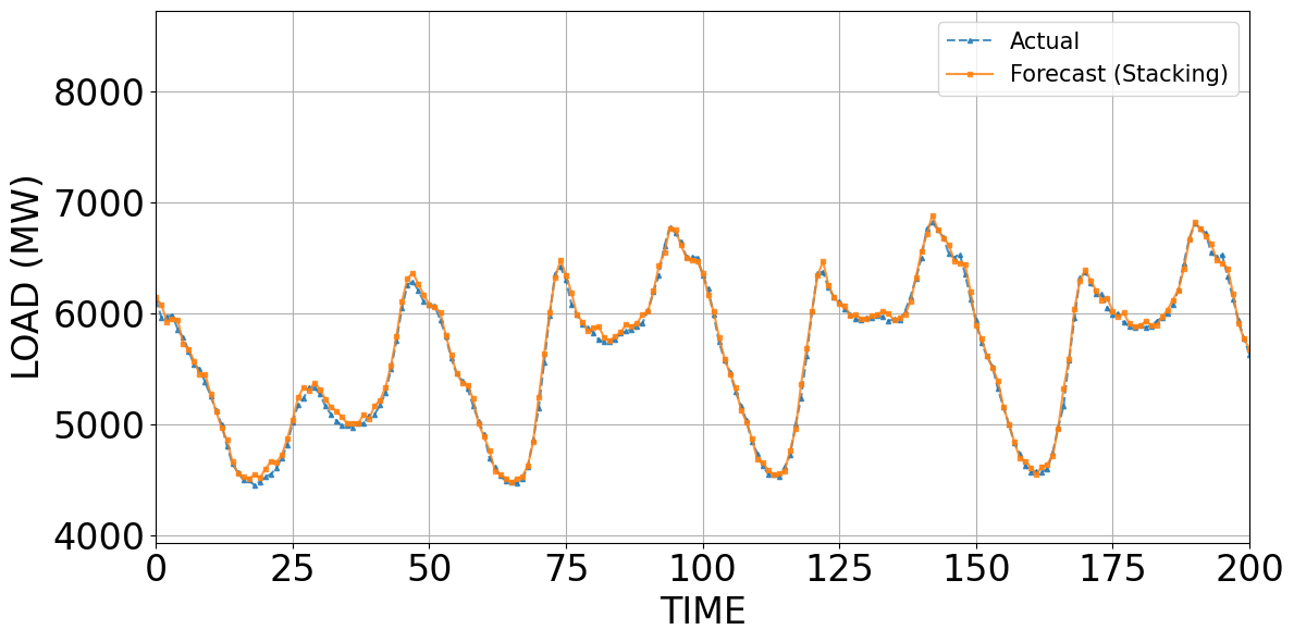
Figure 7. Predicted and actual values using the Stacking model
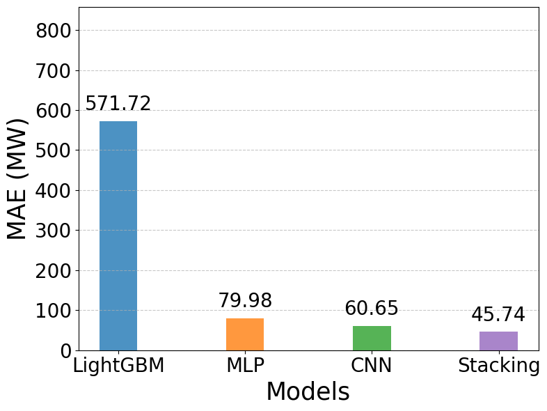
Figure 8. Comparison of MAE values across models (MW)
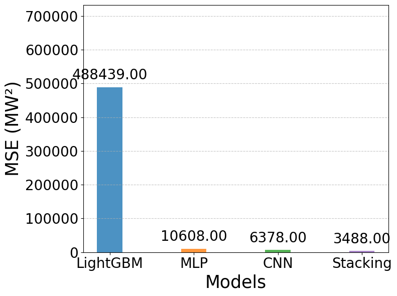
Figure 9. Comparison of MSE values across models (MW2)
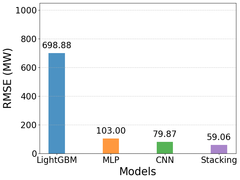
Figure 10. Comparison of RMSE values across models
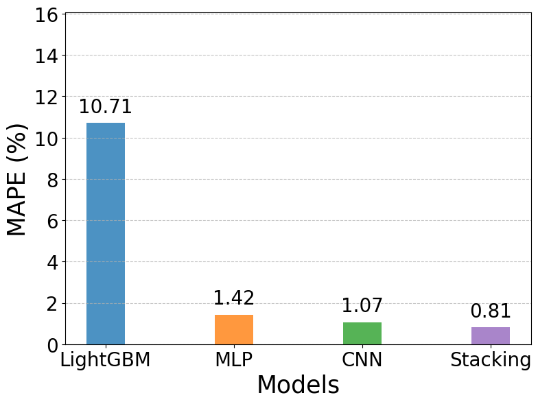
Figure 11. Comparison of MAPE values across models
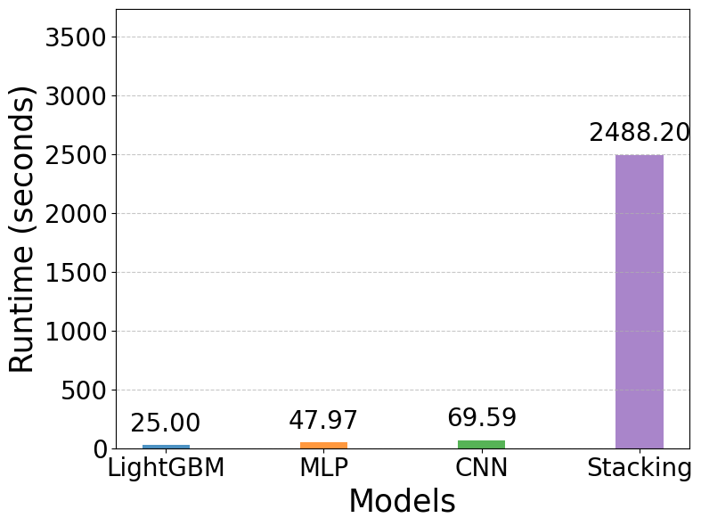
The runtime comparison of the four models is illustrated in Figure 12. Figure 12 illustrates the runtime performance of the four models. The results indicate that LightGBM has the shortest runtime of only 25 seconds, reflecting its computational efficiency and relatively limited forecasting accuracy. The MLP and CNN models require slightly more time, with runtimes of 48 seconds and 70 seconds, respectively, which remain acceptable given their substantially improved accuracy compared to LightGBM. In contrast, the Stacking model demands a considerably higher computational cost, with a runtime of 2,488 seconds. This significant increase in training and inference time is attributed to integrating multiple base learners and the additional complexity of the ensemble framework. All experiments were executed on Google Colab Pro with the High-RAM runtime configuration (approximately 25–30 GB RAM), equipped with an Intel Xeon-class CPU and an NVIDIA Tesla T4 GPU (16 GB VRAM). The runtimes reported in Figure 12 include both training and inference under this hardware environment.
Overall, the findings suggest a clear trade-off between accuracy and computational efficiency. While LightGBM is the fastest model, it produces the least accurate forecasts. Neural network models such as MLP and CNN achieve a balanced compromise, offering relatively short runtimes with markedly improved predictive performance. Stacking provides the most accurate forecasts across all evaluation metrics, but at the expense of substantially longer execution time. This may limit its practical applicability in real-time or near-real-time load forecasting scenarios.
Figure 12. Comparison of Runtime values across models
Discussion
The experimental findings from Figure 4 to Figure 12 reveal distinct behaviors across the forecasting models under investigation. LightGBM, while computationally efficient, is limited to capturing the overall trend of the load series and fails to model short-term fluctuations or extreme values, resulting in higher errors. This reflects the inherent weakness of tree-based models when applied to highly dynamic and periodic time series data. MLP improves substantially by modeling nonlinear relationships and capturing periodic variations, though errors persist at abrupt changes. CNN further advances performance by extracting local temporal features, generating forecasts that align closely with actual profiles. This confirms its superiority in modeling sequential dependencies, consistent with prior works using CNN-based forecasting [47]–[53].
The Stacking model emerges as the best-performing approach, achieving the lowest errors across all metrics by exploiting the complementary strengths of CNN, MLP, and LightGBM. Its effectiveness lies in combining sequence-based learners (CNN) with feature-based learners (MLP, LightGBM), allowing robust modeling of temporal motifs and nonlinear feature interactions. This aligns with recent studies advocating hybrid or ensemble approaches [66]–[69], demonstrating improved robustness compared to single-model baselines. Nonetheless, this superior accuracy comes at the cost of much higher computational complexity (Figure 12), limiting its applicability in real-time contexts.
These observations suggest that no single model is universally optimal. While LightGBM offers speed, it sacrifices accuracy; CNN and MLP provide a balance of accuracy and efficiency; and Stacking achieves the highest accuracy at the expense of runtime. The choice of method should therefore depend on application priorities, whether accuracy, computational speed, or a compromise of both. A limitation of this study is the absence of statistical significance testing, such as the Diebold–Mariano test, which will be addressed in future work. Further research may incorporate richer exogenous inputs (e.g., temperature, holidays), explore hybrid deep learning frameworks (CNN–Transformer), and develop lightweight ensemble variants to reduce execution time.
Table 2. Hyperparameter Search Space for the Proposed Stacking Framework
Model | Hyperparameters | Search Space |
MLP
| Neurons per hidden layer (3 layers) | {16, 32, 64} |
Activation function | {ReLU} |
Learning rate | {0.001} |
Optimizer | {Adam} |
Loss function | {MSE, MAE} |
Batch size | {16, 32, 64} |
Epochs | {100, 200, 300, 400, 500} |
Early stopping patience | {10} |
CNN
| Filters per conv layer (3 layers) | {16, 32, 64} |
Kernel size | {3, 5} |
Activation function | {ReLU} |
Dropout rate | {0.1, 0.2, 0.3} |
Learning rate | {0.001} |
Optimizer | {Adam} |
Loss function | {MSE, MAE} |
Batch size | {16, 32, 64} |
Epochs | {100, 200, 300, 400, 500} |
Early stopping patience | {10} |
LightGBM
| Number of leaves | {31, 63, 127} |
Learning rate | {0.05, 0.1, 0.2} |
n_estimators (boosting rounds) | {100, 300, 500, 1000} |
Max depth | {-1, 10, 20} |
Feature fraction | {0.7, 0.8, 0.9, 1.0} |
Bagging fraction | {0.7, 0.8, 0.9, 1.0} |
Bagging frequency | {1, 5} |
L1 regularization (λ1) | {0, 1, 5, 10} |
L2 regularization (λ2) | {0, 1, 5, 10} |
Meta-Learner (Ridge Regression) | Regularization strength (α) | {0.0001, 0.001, 0.01, 0.1, 1.0} |
Solver | {auto} |
Input features | {OOF predictions of CNN, MLP, LightGBM} |
Stacking Framework
| Cross-validation strategy | TimeSeriesSplit |
Number of folds | {5} |
OOF predictions | {Enabled} |
Final prediction | Weighted combination learned by Ridge |
CONCLUSIONS
This study comprehensively compared four short-term load forecasting models—LightGBM, MLP, CNN, and a hybrid Stacking framework. The main contributions can be summarized as follows: (i) design and evaluation of a stacking ensemble that integrates sequence-based (CNN) and feature-based (MLP, LightGBM) learners through a Ridge meta-learner, (ii) extensive benchmarking against individual baselines across multiple error metrics, and (iii) analysis of the trade-off between accuracy and computational cost in practical forecasting contexts. The results demonstrate that Stacking consistently achieved the best forecasting accuracy, outperforming all baselines across MAE, MSE, RMSE, and MAPE. CNN and MLP provided a strong balance of accuracy and runtime, while LightGBM offered the fastest execution but at the cost of precision. These findings confirm the effectiveness of ensemble learning for short-term load forecasting and highlight that model selection should be application-dependent.
This study also has limitations. The runtime of Stacking is substantially higher, restricting its applicability in real-time operations. In addition, statistical significance testing (e.g., Diebold–Mariano test) was not conducted and will be included in future research. Future work will incorporate richer exogenous inputs (e.g., temperature, calendar events), explore hybrid deep learning architectures such as CNN-Transformer, and develop lightweight ensemble frameworks to preserve accuracy while reducing computational demands. Overall, the proposed stacking approach provides a robust solution for scenarios where accuracy is critical and computational resources are sufficient. At the same time, CNN and MLP are practical alternatives in operational settings. These insights support designing more reliable, efficient, and context-adaptive load forecasting systems for modern power grids.
REFERENCES
- A. Irankhah, S. R. Saatlou, M. H. Yaghmaee, S. Ershadi-Nasab, and M. Alishahi, “A parallel CNN-BiGRU network for short-term load forecasting in demand-side management,” 2022 12th Int. Conf. Comput. Knowl. Eng. ICCKE 2022, pp. 511–516, 2022, https://doi.org/10.1109/ICCKE57176.2022.9960036.
- X. Tang, H. Chen, W. Xiang, J. Yang, and M. Zou, “Short-Term Load Forecasting Using Channel and Temporal Attention Based Temporal Convolutional Network,” Electr. Power Syst. Res., vol. 205, p. 107761, 2022, https://doi.org/10.1016/j.epsr.2021.107761.
- X. Zhang, “Forecasting Short-Term Electricity Load with Combinations of Singular Spectrum Analysis,” Arab. J. Sci. Eng., vol. 48, no. 2, pp. 1609–1624, 2023, https://doi.org/10.1007/s13369-022-06934-y.
- Y. Q. Tan, Y. X. Shen, X. Y. Yu, and X. Lu, “Day-ahead electricity price forecasting employing a novel hybrid frame of deep learning methods: A case study in NSW, Australia,” Electr. Power Syst. Res., vol. 220, p. 109300, 2023, https://doi.org/10.1016/j.epsr.2023.109300.
- A. Oza, D. K. Patel, and B. J. Ranger, “Fusion ConvLSTM-Net: Using Spatiotemporal Features to Increase Residential Load Forecast Horizon,” IEEE Access, vol. 13, pp. 12190–12202, 2025, https://doi.org/10.1109/ACCESS.2025.3528072.
- H. Mansoor and M. Y. Ali, “Spatio-Temporal Short-Term Load Forecasting Using Graph Neural Networks,” 2023 12th Int. Conf. Renew. Energy Res. Appl., pp. 320–323, 2023, https://doi.org/10.1109/ICRERA59003.2023.10269401.
- B. Aksoy and M. Koru, “Estimation of Casting Mold Interfacial Heat Transfer Coefficient in Pressure Die Casting Process by Artificial Intelligence Methods,” Arab. J. Sci. Eng., vol. 45, no. 11, pp. 8969-8980, 2020, https://doi.org/10.1007/s13369-020-04648-7.
- C. Cai, Y. Tao, Q. Ren, and G. Hu, “Short-term load forecasting based on MB-LSTM neural network,” Proc. - 2020 Chinese Autom. Congr. CAC 2020, pp. 5402–5406, 2020, https://doi.org/10.1109/CAC51589.2020.9326696.
- P. Kumar and P. Samui, “Reliability-Based Load and Resistance Factor Design of an Energy Pile with CPT Data Using Machine Learning Techniques,” Arab. J. Sci. Eng., vol. 49, no. 4, pp. 4831-4860, 2023, https://doi.org/10.1007/s13369-023-08253-2.
- A. Jayanth Balaji, B. B. Nair, D. S. Harish Ram, and K. K. George, “A Novel Approach to Faster Convergence and Improved Accuracy in Deep Learning based Electrical Energy Consumption Forecast Models for Large Consumer Groups,” IEEE Access, vol. 13, pp. 15090–15157, 2025, https://doi.org/10.1109/ACCESS.2025.3527863.
- Q. Shen, L. Mo, G. Liu, J. Zhou, Y. Zhang, and P. Ren, “Short-Term Load Forecasting Based on Multi-Scale Ensemble Deep Learning Neural Network,” IEEE Access, vol. 11, pp. 111963–111975, 2023, https://doi.org/10.1109/ACCESS.2023.3322167.
- C. Wei, D. Pi, M. Ping, and H. Zhang, “Short-term load forecasting using spatial-temporal embedding graph neural network,” Electr. Power Syst. Res., vol. 225, p. 109873, 2023, https://doi.org/10.1016/j.epsr.2023.109873.
- A. Sharma and S. K. Jain, “A Novel Two-Stage Framework for Mid-Term Electric Load Forecasting,” IEEE Trans. Ind. Informatics, vol. 20, no. 1, pp. 247–255, 2024, https://doi.org/10.1109/TII.2023.3259445.
- X. Dong, S. Deng, and D. Wang, “A short-term power load forecasting method based on k-means and SVM,” J. Ambient Intell. Humaniz. Comput., vol. 13, no. 11, pp. 5253–5267, 2022, https://doi.org/10.1007/s12652-021-03444-x.
- D. Usman, K. Abdul, and D. Asim, “A Data-Driven Temporal Charge Profiling of Electric Vehicles,” Arab. J. Sci. Eng., vol. 48, no. 11, pp. 15195–15206, 2023, https://doi.org/10.1007/s13369-023-08036-9.
- Y. Liu, Z. Liang, and X. Li, “C,” IEEE Open J. Ind. Electron. Soc., vol. 4, pp. 451–462, 2023, https://doi.org/10.1109/OJIES.2023.3319040.
- M. A. Acquah and Y. Jin, “Spatiotemporal Sequence-to-Sequence Clustering for Electric Load Forecasting,” IEEE Access, vol. 11, pp. 5850–5863, 2023, https://doi.org/10.1109/ACCESS.2023.3235724.
- H. Zhang, Y. Zhang, and Z. Xu, “Thermal Load Forecasting of an Ultra-short-term Integrated Energy System Based on VMD-CNN-LSTM,” Proc. - 2022 Int. Conf. Big Data, Inf. Comput. Network, BDICN 2022, pp. 264–269, 2022, https://doi.org/10.1109/BDICN55575.2022.00058.
- Z. Cai, S. Dai, Q. Ding, J. Zhang, D. Xu, and Y. Li, “Gray wolf optimization-based wind power load mid-long term forecasting algorithm,” Comput. Electr. Eng., vol. 109, p. 108769, 2023, https://doi.org/10.1016/j.compeleceng.2023.108769.
- N. M. M. Bendaoud, N. Farah, and S. Ben Ahmed, “Applying load profiles propagation to machine learning based electrical energy forecasting,” Electr. Power Syst. Res., vol. 203, p. 107635, 2022, https://doi.org/10.1016/j.epsr.2021.107635.
- A. O. Aseeri, “Effective RNN-Based Forecasting Methodology Design for Improving Short-Term Power Load Forecasts: Application to Large-Scale Power-Grid Time Series,” J. Comput. Sci., vol. 68, p. 101984, 2023, https://doi.org/10.1016/j.jocs.2023.101984.
- T. Kavzoglu and A. Teke, “Predictive Performances of Ensemble Machine Learning Algorithms in Landslide Susceptibility Mapping Using Random Forest , Extreme Gradient Boosting ( XGBoost ) and Natural Gradient Boosting ( NGBoost ),” Arab. J. Sci. Eng., vol. 47, no. 6, pp. 7367–7385, 2022, https://doi.org/10.1007/s13369-022-06560-8.
- S. Zhou, Q. Zhang, P. Xiao, B. Xu, and G. Luo, “UniLF: A novel short-term load forecasting model uniformly considering various features from multivariate load data,” Sci. Rep., vol. 15, no. 1, p. 4282, 2025, https://doi.org/10.1038/s41598-025-88566-4.
- S. Ghani, S. Kumari, and S. Ahmad, “Prediction of the Seismic Effect on Liquefaction Behavior of Fine-Grained Soils Using Artificial Intelligence-Based Hybridized Modeling,” Arab. J. Sci. Eng., vol. 47, no. 4, pp. 5411–5441, 2022, https://doi.org/10.1007/s13369-022-06697-6.
- S. Li, J. Wang, H. Zhang, and Y. Liang, “Short-term load forecasting system based on sliding fuzzy granulation and equilibrium optimizer,” Appl. Intell., vol. 53, no. 19, pp. 21606–21640, 2023, https://doi.org/10.1007/s10489-023-04599-0.
- L. Semmelmann, S. Henni, and C. Weinhardt, “Load forecasting for energy communities: a novel LSTM-XGBoost hybrid model based on smart meter data,” vol. 5(Suppl 1), p. 24, 2022. https://doi.org/10.1186/s42162-022-00212-9.
- C. M. Liapis, A. Karanikola, and S. Kotsiantis, “A multivariate ensemble learning method for medium-term energy forecasting,” Neural Comput. Appl., vol. 35, no. 29, pp. 21479–21497, 2023, https://doi.org/10.1007/s00521-023-08777-6.
- W. Zhang, “Short-term Load Forecasting of Power Model Based on CS-Catboost Algorithm,” 2022 IEEE 10th Jt. Int. Inf. Technol. Artif. Intell. Conf., vol. 10, pp. 2295–2299, 2022, https://doi.org/10.1109/ITAIC54216.2022.9836483.
- L. Zhang and D. Jánošík, “Enhanced short-term load forecasting with hybrid machine learning models: CatBoost and XGBoost approaches,” Expert Syst. Appl., vol. 241, 2024, https://doi.org/10.1016/j.eswa.2023.122686.
- C. Zhang, Z. Chen, and J. Zhou, “Research on Short-Term Load Forecasting Using K-means Clustering and CatBoost Integrating Time Series Features,” Chinese Control Conf. CCC, pp. 6099–6104, 2020, https://doi.org/10.23919/CCC50068.2020.9188856.
- R. Panigrahi, N. R. Patne, B. V. Surya Vardhan, and M. Khedkar, “Short-term load analysis and forecasting using stochastic approach considering pandemic effects,” Electr. Eng., vol. 106, no. 3, pp. 3097–3108, 2024, https://doi.org/10.1007/s00202-023-02135-4.
- F. A. Nahid, W. Ongsakul, J. G. Singh, and J. Roy, “Short-term customer-centric electric load forecasting for low carbon microgrids using a hybrid model,” Energy Systems, pp. 1-57. 2024, https://doi.org/10.1007/s12667-024-00704-5.
- N. A. Orka, S. Samit, M. Nazmush, S. Shahi, and A. Ahmed, “Artificial Intelligence-Based Online Control Scheme for the Interconnected Thermal Power Systems Regulations,” Arab. J. Sci. Eng., vol. 48, no. 11, pp. 15153–15176, 2023, https://doi.org/10.1007/s13369-023-07995-3.
- W. Zhang, H. Zhan, H. Sun, and M. Yang, “Probabilistic load forecasting for integrated energy systems based on quantile regression patch time series Transformer,” Energy Reports, vol. 13, no. September 2024, pp. 303–317, 2025, https://doi.org/10.1016/j.egyr.2024.11.057.
- Y. Feng, J. Zhu, P. Qiu, X. Zhang, and C. Shuai, “Short-term Power Load Forecasting Based on TCN-BiLSTM-Attention and Multi-feature Fusion,” Arab. J. Sci. Eng., vol. 50, no. 8, pp. 5475-5486, 2024, https://doi.org/10.1007/s13369-024-09351-5.
- L. Semmelmann, M. Hertel, K. J. Kircher, R. Mikut, V. Hagenmeyer, and C. Weinhardt, “The impact of heat pumps on day-ahead energy community load forecasting,” Appl. Energy, vol. 368, p. 123364, 2024, https://doi.org/10.1016/j.apenergy.2024.123364.
- O. Cagcag Yolcu, H. K. Lam, and U. Yolcu, “Short-term load forecasting: cascade intuitionistic fuzzy time series—univariate and bivariate models,” Neural Comput. Appl., vol. 5, 2024, https://doi.org/10.1007/s00521-024-10280-5.
- W. Yang, S. N. Sparrow, and D. C. H. Wallom, “A comparative climate-resilient energy design: Wildfire Resilient Load Forecasting Model using multi-factor deep learning methods,” Appl. Energy, vol. 368, p. 123365, 2024, https://doi.org/10.1016/j.apenergy.2024.123365.
- B. Zhou, H. Wang, Y. Xie, G. Li, D. Yang, and B. Hu, “Regional short-term load forecasting method based on power load characteristics of different industries,” Sustain. Energy, Grids Networks, vol. 38, 2024, https://doi.org/10.1016/j.segan.2024.101336.
- M. A. Jahin, M. S. H. Shovon, J. Shin, I. A. Ridoy, and M. F. Mridha, “Big Data—Supply Chain Management Framework for Forecasting: Data Preprocessing and Machine Learning Techniques,” Arch. Comput. Methods Eng., vol. 31, no. 6, pp. 3619–3645, 2024, https://doi.org/10.1007/s11831-024-10092-9.
- G. Rozinaj, “Comprehensive Electric load forecasting using ensemble machine learning methods,” 2022 29th Int. Conf. Syst. Signals Image Process., pp. 1–4, 2022, https://doi.org/10.1109/IWSSIP55020.2022.9854390.
- G. F. Fan, R. T. Zhang, C. C. Cao, Y. H. Yeh, and W. C. Hong, “Applications of empirical wavelet decomposition, statistical feature extraction, and antlion algorithm with support vector regression for resident electricity consumption forecasting,” Nonlinear Dyn., vol. 111, no. 21, pp. 20139–20163, 2023, https://doi.org/10.1007/s11071-023-08922-9.
- H. Min, F. Lin, K. Wu, J. Lu, Z. Hou, and C. Zhan, “Broad learning system based on Savitzky – Golay filter and variational mode decomposition for short-term load forecasting,” 2022 IEEE Int. Symp. Prod. Compliance Eng. - Asia, pp. 1–6, https://doi.org/10.1109/ISPCE-ASIA57917.2022.9970794.
- Z. Li and Z. Tian, “Enhancing real-time and day-ahead load forecasting accuracy with deep learning and weighed ensemble approach,” Appl. Intell., vol. 55, no. 4, pp. 1–23, 2025, https://doi.org/10.1007/s10489-024-06155-w.
- Y. Wang, S. Feng, B. Wang, and J. Ouyang, “Deep transition network with gating mechanism for multivariate time series forecasting,” Appl. Intell., vol. 53, no. 20, pp. 24346–24359, 2023, https://doi.org/10.1007/s10489-023-04503-w.
- V. K. Saini, R. Kumar, A. S. Al-Sumaiti, A. Sujil, and E. Heydarian-Forushani, “Learning based short term wind speed forecasting models for smart grid applications: An extensive review and case study,” Electr. Power Syst. Res., vol. 222, p. 109502, 2023, https://doi.org/10.1016/j.epsr.2023.109502.
- G. Memarzadeh and F. Keynia, “Short-term electricity load and price forecasting by a new optimal LSTM-NN based prediction algorithm,” Electr. Power Syst. Res., vol. 192, 2021, https://doi.org/10.1016/j.epsr.2020.106995.
- J.-W. Xiao, X.-Y. Cui, X.-K. Liu, H. Fang, and P.-C. Li, “Improved 3D LSTM: A Video Prediction Approach to Long Sequence Load Forecasting,” IEEE Trans. Smart Grid, vol. 16, no. 2, pp. 1–1, 2024, https://doi.org/10.1109/TSG.2024.3458989.
- K. Song et al., “Short-term load forecasting based on CEEMDAN and dendritic deep learning,” Knowledge-Based Syst., vol. 294, 2024, https://doi.org/10.1016/j.knosys.2024.111729.
- S. Deng, X. Dong, L. Tao, J. Wang, Y. He, and D. Yue, “Multi-type load forecasting model based on random forest and density clustering with the influence of noise and load patterns,” Energy, vol. 307, 2024, https://doi.org/10.1016/j.energy.2024.132635.
- T. Zhang, Y. Huang, H. Liao, and Y. Liang, “A hybrid electric vehicle load classification and forecasting approach based on GBDT algorithm and temporal convolutional network,” Appl. Energy, vol. 351, p. 121768, 2023, https://doi.org/10.1016/j.apenergy.2023.121768.
- D. A. Khan, A. Arshad, and Z. Ali, “Performance Analysis of Machine Learning Techniques for Load Forecasting,” ICET 2021 - 16th Int. Conf. Emerg. Technol. 2021, Proc., pp. 1–6, 2021, https://doi.org/10.1109/ICET54505.2021.9689903.
- J. Shi, W. Zhang, Y. Bao, D. W. Gao, and Z. Wang, “Load Forecasting of Electric Vehicle Charging Stations: Attention Based Spatiotemporal Multi-Graph Convolutional Networks,” IEEE Trans. Smart Grid, vol. PP, no. 8, p. 1, 2023, https://doi.org/10.1109/TSG.2023.3321116.
- A. Khaleghi and H. Karimipour, “A Probabilistic-Based Approach for Detecting Simultaneous Load Redistribution Attacks Through Entropy Analysis and Deep Learning,” IEEE Trans. Smart Grid, vol. 16, no. 2, pp. 1851–1861, 2024, https://doi.org/10.1109/TSG.2024.3524455.
- B. Chen, W. Yang, B. Yan, and K. Zhang, “An advanced airport terminal cooling load forecasting model integrating SSA and CNN-Transformer,” Energy Build., vol. 309, p. 114000, 2024, https://doi.org/10.1016/j.enbuild.2024.114000.
- A. Stratman, T. Hong, M. Yi, and D. Zhao, “Net Load Forecasting with Disaggregated Behind-the-Meter PV Generation,” IEEE Trans. Ind. Appl., vol. 59, no. 1, pp. 5341–5351, 2023, https://doi.org/10.1109/TIA.2023.3276356.
- A. Mystakidis et al., “Energy generation forecasting: elevating performance with machine and deep learning,” Computing, vol. 105, no. 8, pp. 1623–1645, 2023, https://doi.org/10.1007/s00607-023-01164-y.
- M. Alkasassbeh and S. A. Baddar, “Intrusion Detection Systems : A State-of-the-Art Taxonomy and Survey,” Arab. J. Sci. Eng., vol. 48, no. 8, pp. 10021–10064, 2023, https://doi.org/10.1007/s13369-022-07412-1.
- W. Tercha, S. A. Tadjer, and F. Chekired, “Machine Learning-Based Forecasting of Temperature and Solar Irradiance for Photovoltaic Systems,” Energies, vol. 17, no. 5, p. 1124, 2024, https://doi.org/10.3390/en17051124.
- U. Sencan and G. S. N. Arica, “Forecasting of Day-Ahead Electricity Price Using Long Short-Term Memory-Based Deep Learning Method,” Arab. J. Sci. Eng., vol. 47, no. 11, pp. 14025–14036, 2022, https://doi.org/10.1007/s13369-022-06632-9.
- P. Nedić, I. Djurović, M. Ćalasan, S. Kovačević, and K. Pavlović, “Electrical energy load forecasting using a hybrid N-BEATS - CNN Approach: Case study Montenegro,” Electr. Power Syst. Res., vol. 247, p. 111749, 2025, https://doi.org/10.1016/j.epsr.2025.111749.
- W. Lin, D. Wu, and M. Jenkin, “Electric Load Forecasting for Individual Households via Spatial-temporal Knowledge Distillation,” IEEE Trans. Power Syst., vol. 40, no. 1, pp. 572–584, 2024, https://doi.org/10.1109/TPWRS.2024.3393926.
- R. Tian, J. Wang, Z. Sun, J. Wu, X. Lu, and L. Chang, “Multi-Scale Spatial-Temporal Graph Attention Network for Charging Station Load Prediction,” IEEE Access, vol. 13, pp. 29000–29017, 2025, https://doi.org/10.1109/ACCESS.2025.3541118.
- H. Wang, J. D. Watson, and N. R. Watson, “A Lyapunov-based nonlinear direct power control for grid-side converters interfacing renewable energy in weak grids,” Electr. Power Syst. Res., vol. 221, p. 109408, 2023, https://doi.org/10.1016/j.epsr.2023.109408.
- N. B. Vanting, Z. Ma, and B. N. Jørgensen, “Evaluation of neural networks for residential load forecasting and the impact of systematic feature identification,” Energy Informatics, vol. 5, no. 4, pp. 1–24, 2022, https://doi.org/10.1186/s42162-022-00224-5.
- H. Hu, Z. Cheng, and H. Fan, “Short-term load forecasting method based on deep learning under digital driving,” In 2022 Asian Conference on Frontiers of Power and Energy (ACFPE), pp. 188-192, pp. 188–192, 2024, https://doi.org/10.1109/ACFPE56003.2022.9952181.
- B. Mechanism, J. Xiao, P. Liu, H. Fang, and X. Liu, “Short-Term Residential Load Forecasting With Baseline-Refinement Profiles and,” IEEE Trans. Smart Grid, vol. 15, no. 1, pp. 1052–1062, 2024, https://doi.org/10.1109/TSG.2023.3290598.
- Y. Ding, C. Huang, K. Liu, P. Li, and W. You, “Short-term forecasting of building cooling load based on data integrity judgment and feature transfer,” Energy Build., vol. 283, p. 112826, 2023, https://doi.org/10.1016/j.enbuild.2023.112826.
- S. V. Oprea and A. Bâra, “On-grid and off-grid photovoltaic systems forecasting using a hybrid meta-learning method,” Knowl. Inf. Syst., vol. 66, no. 4, pp. 2575–2606, 2024, https://doi.org/10.1007/s10115-023-02037-8.
AUTHOR BIOGRAPHY

| Trung Dung Nguyen was born in 1976 in Vietnam. He received a Master’s degree in Electrical Engineering from Ho Chi Minh City University of Technology and Education, Vietnam, in 2017. He lectures at the Faculty of Electrical Engineering Technology, Industrial University of Ho Chi Minh City, Ho Chi Minh City, Vietnam. His research focuses on applications of metaheuristic algorithms in power system optimization, optimal control, and model predictive control. Email: nguyentrungdung@iuh.edu.vn |
|
|

| Nguyen Anh Tuan     received a B.Sc. degree from the Industrial University of Ho Chi Minh City, Vietnam 2012, and an M.Sc. degree from the HCMC University of Technology and Education, Vietnam, in 2015. He is a Lecturer with the Faculty of Electrical Engineering Technology at the Industrial University of Ho Chi Minh City, Vietnam. His main research interests include power quality and load forecasting. received a B.Sc. degree from the Industrial University of Ho Chi Minh City, Vietnam 2012, and an M.Sc. degree from the HCMC University of Technology and Education, Vietnam, in 2015. He is a Lecturer with the Faculty of Electrical Engineering Technology at the Industrial University of Ho Chi Minh City, Vietnam. His main research interests include power quality and load forecasting. Email: nguyenanhtuan@iuh.edu.vn |
Trung Dung Nguyen (Hybrid Stacking of Multilayer Perceptron, Convolutional Neural Network, and Light Gradient Boosting Machine for Short-Term Load Forecasting)