ISSN: 2685-9572 Buletin Ilmiah Sarjana Teknik Elektro
Vol. 7, No. 4, December 2025, pp. 756-773
Optimal PID Controller Based on Different Modified Grasshopper Optimization Algorithm for Nonlinear
Single-Input Single-Output System
Aliaa A. Flaih 1, Ekhlas H. Karam 2, Yousra A. Mohammed 3
1 Mustansiriyah University, Baghdad, Iraq.
2 Department of Computer Engineering, Mustansiriyah University, Baghdad, Iraq.
3 College of Communication Engineering, University of Technology, Baghdad, Iraq.
ARTICLE INFORMATION |
| ABSTRACT |
Article History: Received 20 August 2025 Revised 19 October 2025 Accepted 03 November 2025 |
| 
This paper presents a comparative study of the Grasshopper Optimization Algorithm (GOA) with three suggested modified versions—Levy Flight GOA (LFGOA), Dynamic Attraction-Repulsion GOA (DARGOA), and Chaotic GOA (CHGOA)—for tuning Proportional-Integral-Derivative (PID) controller parameters in a nonlinear Single-Input Single-Output (SISO) system. The research contribution is the development and evaluation of CHGOA, which aims to improve convergence speed and transient response stability. The methodology employs exploratory and exploitative mechanisms of each algorithm to optimize PID parameters based on six objective functions. Performance metrics include rise time, settling time, overshoot, peak value, and best fitness obtained from MATLAB/Simulink simulations. A second-order Mass-Spring-Damper (MSD) system is used as a representative nonlinear SISO system. Simulation results indicate that the proposed CHGOA consistently achieves lower fitness values, faster convergence, and stable transient responses compared to LFGOA, DARGOA, and standard GOA, under the tested objective functions. While LFGOA and DARGOA show competitive performance in traditional error metrics, standard GOA exhibits slower convergence in simulation scenarios. In this paper, the performance of the MSD system controlled by the proposed optimal PID with GOAs was also compared with the performance of this system with Nonlinear PIDs (NPIDs) which proposed by previous studies. The comparison results showed the efficiency of our proposed controllers in improving the performance of the MSD system, especially the CHGOA. Overall, the proposed CHGOA provides an effective balance between error minimization, convergence speed, and transient response performance, making it suitable for high-precision real-time applications. |
Keywords: PID Controller; Dynamically Attraction-Repulsion Grasshopper Optimization Algorithm; Nonlinear Mass-Spring Damper; Lévy Flight and Chaotic Grasshopper Optimization Algorithm; Benchmark Functions CEC2017; Linear And Nonlinear Desired Inputs |
Corresponding Author: Yousra A. Mohammed, College of communication, University of Technology- Baghdad, Iraq. Email: yousra.a.mohammed@uotechnology.edu.iq |
This work is licensed under a Creative Commons Attribution-Share Alike 4.0 
|
Document Citation: A. A. Flaih, E. H. Karam, and Y. A. Mohammed, “Optimal PID Controller Based on Different Modified Grasshopper Optimization Algorithm for Nonlinear Single-Input Single-Output System,” Buletin Ilmiah Sarjana Teknik Elektro, vol. 7, no. 4, pp. 756-773, 2025, DOI: 10.12928/biste.v7i4.14394. |
- INTRODUCTION
The nonlinear Single-Input Single-Output (SISO) systems represent a significant challenge in control engineering due to their inherent complexity and the difficulty of modeling them accurately using conventional techniques. Such systems exhibit nonlinear behaviors that limit the effectiveness of classical linear control methods. These systems appear in many industrial and engineering applications, including the control of electric motors, mechanical systems with nonlinear friction, and aerodynamic processes.
Generally, nonlinear SISO systems are addressed through two main approaches: linear approximation and nonlinear control. In some cases, the system can be linearized around a specific operating point, enabling the application of established techniques such as Model Predictive Control (MPC) [1]–[3], Linear Quadratic Gaussian (LQG) [4][5], and Proportional-Integral-Derivative (PID) control [6][7]. However, when the system exhibits strong nonlinearities or requires operation across a wide range of conditions, more advanced control methods are necessary. These include Model Reference Control (MRC) with Fuzzy Logic [8][9] and adaptive Sliding Mode Control (SMC) [10]–[12], which offer enhanced robustness and better handling of unexpected disturbances and parameter variations.
Optimization techniques have become fundamental tools for finding optimal controller parameters to improve system performance, minimize error, and ensure stability. In particular, metaheuristic algorithms have gained increasing attention due to their capability to automatically tune controller parameters for nonlinear SISO systems, especially PID controllers. For example, Praveen Kumar et al. [13] introduced a PID controller design based on the Cuckoo Optimization Algorithm (COA), successfully applied to nonlinear systems such as the inverted pendulum, ship roll dynamics, and the Van der Pol Oscillator (VDPO). Hazem I. Ali et al. [14] designed an optimal nonlinear controller based on the model reference approach, optimized with the Invasive Weed Optimization (IWO) algorithm, and validated on the ball and plate system, showing improved robustness and performance. However, conventional metaheuristic algorithms may suffer from limitations such as slow convergence, premature entrapment in local optima, and an insufficient balance between exploration and exploitation [15]–[17]. To overcome these limitations, several algorithmic enhancements have been proposed. Vishal Srivastava et al. [18] introduced hybrid optimization approaches by integrating Particle Swarm Optimization with the Gravitational Search Algorithm (PSO-GSA) and with the Grey Wolf Optimizer (PSO-GWO) for tuning PID controllers in nonlinear systems such as the Continuous Stirred Tank Reactor (CSTR), inverted pendulum, and blood glucose regulation models. Vijayakumar Kaliappan [19] developed an Enhanced Genetic Algorithm (EGA)-based PID controller to regulate nonlinear closed-loop CSTR systems, demonstrating improved performance over conventional approaches through simulation. Furthermore, Zijing Chu et al. [20] presented a novel PID tuning approach integrating Whale Optimization Algorithm (WOA) with Backpropagation (BP) neural networks for nonlinear and time-varying problems, achieving fast response, improved stability, reduced overshoot, and high control precision. The Grasshopper Optimization Algorithm (GOA), inspired by grasshopper swarming behavior, has been enhanced through the integration of Lévy flight mechanisms into its structure, leading to the development of the Lévy Flight GOA (LFGOA), which improves global exploration, accelerates convergence, and enhances solution accuracy in engineering optimization problems [21][22]. Furthermore, the combination of chaotic maps with swarm-based optimizers has demonstrated robust performance improvements. For instance, a hybrid Particle Swarm Optimization–Gravitational Search Algorithm (PSO–GSA) incorporating chaotic mapping achieved superior robustness in H₂/H∞ control design for generator-based systems [23].
This study builds upon these insights by proposing three modified variants of GOA that incorporate Lévy Flight GOA (LFGOA), Chaotic (CHGOA), and Dynamic Attraction-Repulsion (DARGOA). both the original and the improved variants of the GOA are employed to tune the PID controller parameters to enhance convergence speed, superior stability, robustness, and control accuracy of nonlinear SISO system. in this paper a second order Mass-Spring Damper (MSD) was considerd as an example of SISO nonlinear system. The suggested optimization algorithms are initially evaluated using the CEC2017 benchmark functions to validate their optimization performance. The optimization process considers six objective functions. These functions allows for a comprehensive comparison between the original and the modified GOA versions, highlighting the improvements achieved through algorithmic modifications.
The rest of this paper is organized as follows, the origin GOA and the suggested modified GOAs are given in section 2, the fitness function types are detailed in section 3, the Benchmark functions (CEC2017) are illustrated and performance analysis in Section 4, designing an optimal PID controller for nonlinear SISO system is explained in Section 5, the simulation results and analysis are shown in Section 6, and the conclusions are presented in Section 7.
- GRASSHOPPER OPTIMIZATION ALGORITHM AND SUGGESTED MODIFICATION METHODS
Optimization refers to the process of determining the best solution to a given problem by improving the characteristics of a cost function and achieving the global optimum. Population-based, or metaheuristic, optimization methods are stochastic approaches that explore the search space through multiple candidate solutions (agents). Many of these stochastic strategies are inspired by natural phenomena, where the collective behaviors of animals and insects such as birds, ants, grasshoppers, flies, and even microorganisms are modeled, and are therefore categorized as Nature-Inspired Algorithms. One of the optimization algorithms techniques is Grasshopper Optimization Algorithm. This method is introduced by Saremi et al. [24], a novel and intriguing swarm intelligence technique that mimics the foraging and swarming behavior of grasshoppers. These insects significantly impact crop production and agriculture [25][26]. The mathematical modeling of this behavior is expressed through the position update mechanism represented in Eq. (1), which defines how grasshoppers interact and adjust their positions based on social forces and environmental influences.
| 
| (1) |
 is distance between two grasshoppers
  and
and  ,
,  is social force function computed as follows:
| 
| (2) |
As expressed in above equation, the position of the  grasshopper at iteration t+1 denoted by
  is updated according to the interactions among individuals and the target position. In this formulation,
  represents the strength of attraction between grasshoppers, while l defines the attraction length. The search boundaries for each dimension are limited by the lower and upper bounds,
  and
and  . The term
  corresponds to the target location in the d-dimensional search space. Furthermore, the shrinking coefficient c is employed to gradually reduce the comfort zone, ensuring a balance between exploration and exploitation during the optimization process.
| 
| (3) |
where  is the maximum value,
  is the value of minimum,
  is the current iteration, and
  indicates the maximum number of iterations.
The optimization process in GOA begins by initializing a set of candidate solutions, where each grasshopper’s position corresponds to a design variable vector. During the search, these positions are iteratively updated according to Eq. (1) to Eq. (3), while the best-performing individual is continuously tracked. This evolutionary mechanism is repeated until the termination criterion is satisfied, at which point the position of the best grasshopper is considered the optimal solution. In the following subsections, the three suggested methods to modify the origin GOA are explained. These methods are Lévy Flight GOA (LFGOA), Dynamically Attraction–Repulsion GOA (DARGOA), and Chaotic GOA (CHGOA).
- Modified Grasshopper Optimization Algorithm Based on Lévy Flight
Lévy flight [27] is a mathematical model that facilitates random search behavior with occasional long jumps, making it particularly effective for enhancing exploration in optimization algorithms. Due to the complexity of its exact implementation, an approximated simulation is used here as follows:
| 
| (4) |
Here,  denotes the problem dimension, while
  and
and  are two uniformly distributed random variables within the interval [0, 1]. The parameter
  is a constant set to 1.5 as suggested by S. Mirjalili [28], and
  is computed using the following expression:
| 
| (5) |
where 
In this work, the original GOA is modified by incorporating the Lévy Flight mechanism directly into the core position update formula. Specifically, a subset of 50% of the search agents is guided to perform Lévy-based movements when no better neighboring solutions are identified. This adjustment aims to increase exploration capability and reduce the risk of premature convergence. Unlike prior works [29][30] where Lévy steps are often implemented as external modifications or separate random walks, the proposed modification applies the Lévy jump directly within the attraction-repulsion formula on Eq. (1). This integration enhances the algorithm's ability to escape local optima while maintaining a balance between diversification and intensification. The mathematical formulation of the Lévy jump is defined as follows:
| 
| (6) |
where agents satisfying:
| 
| (7) |
where  is number of agents are selected to undergo the Lévy-based update.
- Modified Grasshopper Optimization Algorithm Based on Dynamically Attraction–Repulsion
In order to achieve a more effective trade-off between the exploration and exploitation phases within the GOA, a dynamic modification of the attraction () and repulsion ( ) coefficients is introduced. Unlike the standard GOA in Eq. (2), which uses fixed values ( = 0.5 and = 1.5) as proposed by S. Mirjalili in [28], this approach employs linearly time-varying parameters defined as follows:
| 
| (8) |
| 
| (9) |
Where is the current iteration and is the maximum number of iterations. The parameter ranges were selected based on both the original GOA constants and empirical testing:
 = 0.5: consistent with the original GOA to ensure strong initial attraction
 = 0.1: to gradually reduce inter-agent attraction near convergence.
 = 1.5: default repulsion distance in the original model.
 = 0.5: reduces the repulsion effect at later iterations for better convergence.
This modification is inspired by a recent study [31], which employed time-varying parameters to gradually reduce the interaction zone among agents, thereby improving convergence and limiting excessive exploration.
- Modified Grasshopper Optimization Algorithm Based on Chaotic
To achieve a better trade-off between exploration and exploitation in the original GOA, the primary position update equation (Eq. (1)) is refined through the incorporation of a chaotic term based on the Logistic Map. The logistic map is a well-known nonlinear function that produces chaotic behavior and has been widely used to diversify search trajectories and avoid premature convergence [32], where logistic map equation is defined as follows:
| 
| (10) |
where the control parameter  is assigned a value of 4 to ensure the generation of random numbers within the interval (0, 1) [32].
In this work, we directly embed the logistic value into the attraction–repulsion term of the position update formula, instead of using chaos for initial population or parameter control as done in prior works [33]. The modified position update equation is given by:
| 
| (11) |
As illustrate in Eq. (11) subsections, the modification to the original GOA (LFGOA, DARGOA, and CHGOA) are suggested to address specific performance limitations, including premature convergence, imbalance between exploration and exploitation, and adaptation to complex search landscapes. To consolidate these enhancements and facilitate a direct step-by-step comparison with the baseline algorithm, all versions were reformulated into a unified pseudo-code framework. This integration not only standardizes the representation but also allows for clear identification of the operational differences between the original GOA and its variants. Specifically, Table 1 provides the complete modified unified pseudo-code, where the first column outlines the original GOA steps, and the following columns detail the corresponding modifications applied in LFGOA, DARGOA, and CHGOA.
Table 1. Unified Pseudo-code for Original GOA with Three Modifications.
Step | Original GOA | LFGOA (GOA + Lévy flight) | DARGOA (Adaptive &  ) ) | CHGOA (Logistic Map) | Remark |
1 | Initialize population  randomly within [, ], i = 1...N randomly within [, ], i = 1...N | Same as Original | Same as Original | Same as Original | - |
2 | Initialize parameters F = 0.5, l = 1.5, , | Same | Adapt F and l dynamically in Step 5.2 | Same | Parameter adaptation in DARGOA |
3 | Evaluate fitness  = fobj( = fobj( ) )
| Same | Same | Same | - |
4 | Set best solution  = min ( = min ( ) ) | Same | Same | Same | - |
5 | While j < : | Same | Same | Same | Iterative update loop |
5.1 | Update shrinking factor: | Same | Same | Same | - |
5.2 | Update positions: Eq. (1) with s(r) | Same + Lévy flight:  
| Adapt F and l dynamically  , ,

| Replace Eq. (1) to Eq. (11) | Main differences occur here |
5.3 | Boundary check: ∈ [, ] | Same | Same | Same | - |
5.4 | Evaluate fitness = fobj() | Same | Same | Same | - |
5.5 | Update best solution: if <  : = , = : = , = | Same | Same | Same | - |
6 | End While | Same | Same | Same | Termination condition met |
- FITNESS FUNCTION TYPES
Designing any type of controller requires the determination of optimal control parameters. Accordingly, specific parameters must be calculated to minimize the chosen objective function. It is important to note that, since the system error is generally time-dependent, multiple performance indices are needed to comprehensively evaluate controller performance. Several fitness functions are widely employed in control optimization, including the Integral of Squared Time multiplied by Squared Error (ISTSE), Integral Squared Error (ISE), Integral of Squared Time multiplied by Error Squared (ISTES), Integral Absolute Error (IAE), Integral of Time multiplied by Squared Error (ITSE), and Integral of Time multiplied by Absolute Error (ITAE). The mathematical formulations of these performance indices are presented in the equations of these functions are [34]–[37]:
- PERFORMANCE ANALYSIS ON CEC2017 BENCHMARK FUNCTIONS AND EVALUATION OF SUGGESTED METHODS
The CEC2017 benchmark suite contains 23 functions, as detailed in Table A1 to Table A3 in Appendix A [38]. In these tables, (Range) denotes the search space boundaries, (D) represents the dimensionality of each function, and ( ) indicates the known global optimum. All benchmark functions are formulated as minimization problems and are categorized into three types: unimodal functions (F1–F7), multimodal functions (F8–F13), and fixed-dimension multimodal functions (F14–F23) [33]. In the present study, to ensure a rigorous and fair comparison, each algorithm was executed 30 independent times on every benchmark function, with a population size of 50 and a maximum of 500 iterations. The performance of each algorithm was assessed by evaluating the mean and standard deviation of the obtained solutions, where lower values correspond to higher robustness and stability in achieving global optimization.
A series of experiments were conducted on a selected set of CEC2017 benchmark functions: F1, F3, F5, F9, F12, F15, F22, and F23. These functions were carefully chosen due to their diverse characteristics, including unimodal, multimodal, hybrid, and composition functions, providing a comprehensive and challenging environment to evaluate the algorithms exploration, exploitation, convergence speed, and solution accuracy capabilities. The performance evaluation involved the original GOA alongside three suggested enhancements: CHGOA, DARGOA, and LFGOA. These variants aim to improve the exploration-exploitation balance, enhance the quality of search in later stages, and reduce the likelihood of premature convergence to local optima. All experiments were conducted under uniform settings regarding population size, number of iterations, and independent runs to ensure a fair and reliable comparison. The results from the comparative performance Table 2 indicate that CHGOA outperforms other algorithms across most functions, especially complex multimodal ones such as F1, F3, and F5, achieving best values near the global optimum with low standard deviation, indicating high accuracy and consistent stability across runs. DARGOA ranks second overall, showing notable improvements over the baseline GOA by reducing mean and standard deviation values, reflecting greater reliability and steadiness. LFGOA demonstrated strong and stable performance particularly on complex composition functions like F22 and F23, attaining the best values and lowest ranks, which indicates its superior capability to explore intricate search spaces precisely. Conversely, the original GOA exhibited variable performance, often ranking in mid to lower positions, underscoring the necessity of the applied enhancements. Moreover, the convergence curves for each benchmark function are presented in Figure 1.
Table 2. Statistical results of benchmark functions for original GOA with three modifications.
Funct-ion | Algorithm | Best | Mean | Median | Worst | Std | Rank |
F1 | LFGOA | 5.1597e+04 | 6.6415e+04 | 6.7461e+04 | 7.9099e+04 | 6.2309e+03 | 4 |
DARGOA | 4.0068e+04 | 6.2679e+04 | 6.2994e+04 | 7.2843e+04 | 6.9920e+03 | 2 |
CHGOA | 3.5531e-09 | 3.3045e-05 | 3.1548e-05 | 8.9628e-05 | 2.4074e-05 | 1 |
GOA | 4.6765e+04 | 6.3980e+04 | 6.4823e+04 | 7.5011e+04 | 7.0392e+03 | 3 |
F3 | LFGOA | 7.5126e+04 | 1.3213e+05 | 1.3347e+05 | 1.8469e+05 | 2.9103e+04 | 4 |
DARGOA | 5.2373e+04 | 1.1605e+05 | 1.1570e+05 | 2.1691e+05 | 3.7302e+04 | 2 |
CHGOA | 2.4606e-07 | 1.1741e-04 | 1.2276e-04 | 2.6940e-04 | 6.8568e-05 | 1 |
GOA | 5.4643e+04 | 1.2786e+05 | 1.2869e+05 | 1.9218e+05 | 3.6305e+04 | 3 |
F5 | LFGOA | 1.5271e+08 | 2.3258e+08 | 2.3265e+08 | 2.9188e+08 | 3.6792e+07 | 3 |
DARGOA | 1.2700e+08 | 2.3000e+08 | 2.4119e+08 | 2.9766e+08 | 4.0783e+07 | 2 |
CHGOA | 28.7968 | 28.8659 | 28.8667 | 28.9126 | 0.0306 | 1 |
GOA | 1.7801e+08 | 2.4519e+08 | 2.4757e+08 | 2.9968e+08 | 3.4426e+07 | 4 |
F9 | LFGOA | 13.4004 | 69.3096 | 51.0655 | 233.3008 | 51.4547 | 2 |
DARGOA | 87.6969 | 170.3005 | 153.6646 | 299.6026 | 54.3970 | 4 |
CHGOA | 0.0038 | 0.0090 | 0.0091 | 0.0153 | 0.0026 | 1 |
GOA | 18.3995 | 73.8144 | 61.3623 | 201.3240 | 42.0337 | 3 |
F12 | LFGOA | 2.5742e+08 | 5.0402e+08 | 5.1791e+08 | 6.9529e+08 | 1.2279e+08 | 3 |
DARGOA | 3.4466e+08 | 5.0375e+08 | 5.0111e+08 | 7.1863e+08 | 1.0722e+08 | 2 |
CHGOA | 0.0521 | 0.1405 | 0.1317 | 0.3733 | 0.0654 | 1 |
GOA | 1.8904e+08 | 5.0483e+08 | 5.1512e+08 | 7.4218e+08 | 1.2790e+08 | 4 |
F15 | LFGOA | 4.3107e-04 | 0.0067 | 7.8390e-04 | 0.0565 | 0.0124 | 3 |
DARGOA | 7.5883e-04 | 0.0139 | 0.0181 | 0.0594 | 0.0153 | 4 |
CHGOA | 3.1152e-04 | 0.0018 | 3.2116e-04 | 0.0209 | 0.0052 | 1 |
GOA | 3.0831e-04 | 0.0065 | 0.0015 | 0.0297 | 0.0093 | 2 |
F22 | LFGOA | -10.4024 | -7.0453 | -7.7596 | -2.7516 | 3.5087 | 1 |
DARGOA | -10.4010 | -6.9423 | -7.7272 | -1.8360 | 3.5728 | 2 |
CHGOA | -10.2162 | -5.3139 | -4.9705 | -2.6177 | 1.5397 | 4 |
GOA | -10.4023 | -5.8027 | -5.0864 | -1.8376 | 3.2334 | 3 |
F23 | LFGOA | -10.5355 | -7.7665 | -10.5289 | -2.4216 | 3.7485 | 1 |
DARGOA | -10.5354 | -7.0533 | -7.8201 | -1.6758 | 3.6411 | 2 |
CHGOA | -10.1022 | -5.2489 | -5.0077 | -2.7597 | 1.2524 | 4 |
GOA | -10.5353 | -6.6485 | -5.1512 | -2.4217 | 3.7845 | 3 |
Figure 1. Convergence characteristics of the modified and baseline optimization algorithms on eight detailed benchmark functions
- OPTIMAL PID CONTROLLER DESIGN FOR SISO NONLINEAR MSD SYSTEM
In this study, the Mass spring Damper (MSD) system is adopted as a representative nonlinear SISO plant to validate the effectiveness of optimization approaches for PID tuning by GOA and the modified GOA methods. The MSD system shown in Figure 2 is a mechanical standard benchmark in control theory for vibration dynamics, it can be described as follows [39][40]:
| 
| (18) |
The parameters of this system are listed in Table 3.
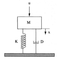
Figure 2. Nonlinear MSD system [40]
Table 3. Model parameters of MSD [40]
Symbol | Description | Value |
M | mass | 1.0 |
g(x, | the nonlinear or uncertain term with respect to the spring, g(x, ( ( x+ x+ ) ) | 

|
f(x) | the nonlinear or uncertain term with respect to the damper, f(x)  x + x +  | 

|

| the nonlinear term with respect to the input term 
| 
|
x | 
| 
|

|  [-b b], b [-b b], b
| 
|
u | Force control signal | … |
Then, Eq. (18) can be rewritten as follows:
| 
| (19) |
The state-space representation of the Eq. (19) is expressed as:
| 
| (20) |
The control law of the PID controller is given by:
| 
| (21) |
where  ,
,  , and
, and  are the proportional, integral, and derivative gains, respectively. The six performance indices IAE, ISE, ISTES, ISTSE, ITAE, and ITSE are used as fitness functions to evaluate the quality of the PID tuning for MSD system.
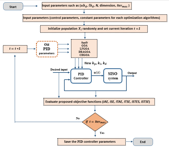
Figure 3 provide a clearer understanding of the interaction between the optimal PID controller and the MSD system and illustrates the step-by-step procedure: starting with the initialization of control parameter bounds, followed by the configuration of the optimization algorithm settings, and finally the evaluation of the MSD system response under the optimized PID controller.
Figure 3. Flowchart of designing optimal PID tuned by modified GOAs for nonlinear MSD system
- SIMULATION RESULT AND ANALYSIS
In this section, a comprehensive analysis is conducted on the performance of the SISO nonlinear MSD system regulated by a PID controller optimized by original GOA and the three suggested modified methods (LFGOA, DARGOA, and CHGOA). A series of simulation tests is carried out to evaluate and compare the effectiveness of each optimization approach in achieving precise and stable control performance. Unity step reference signal is assigned to ensure consistency across all trials. The system parameters adopted in the simulations are listed in Table 4, while Table 5 summarizes the PID controller parameters obtained by each algorithm to maintain the actual system output at the desired reference.
Figure 4 displays the convergence curves for selected benchmark functions, clearly showing the performance differences among the four algorithms, while the bar chart in Figure 5 provides a comparative view of the best fitness values obtained in PID tuning tasks. Across most fitness functions, CHGOA demonstrated a clear advantage in minimizing the best fitness values, as reflected in benchmark results such as F1, F3, F5, F9, F12, and F15, where it consistently achieved the top rank. On the other hand, GOA generally performed on par with LFGOA and DARGOA in basic error metrics but lagged behind in more complex benchmark functions (F1–F15), indicating a relatively slower convergence in highly nonlinear optimization landscapes. Nevertheless, GOA maintained consistent stability, which may be advantageous in systems with strict robustness requirements. The simulation results to evaluate the performance of the controlled nonlinear MSD system for linear and nonlinear desired input are illustrate in the following subsections
Table 4. Input parameters for optimization methods
Optimization methods | Parameters | Values |
All | dimension | 3 |
lower value for , , | [40,2,8] |
upper value for , , | [50,6,12] |
| 25 |
number of populations | 25 |
GOA | intensity of attraction ( ), attractive length scale ( ), attractive length scale ( ) ) | 0.5, 1.5 |
LFGOA | , are random numbers in [0,1],  |
DARGOA | = 0.5, = 0.1, = 1.5, = 0.5 |
CHGOA | = 4,  = 0.1 = 0.1 |
Table 5. Optimal PID parameters obtained by the optimization methods
Algorithm | Fitness |
|
|
|
LFGOA | IAE | 50.0 | 4.73047 | 8.0 |
ISE | 50.0 | 5.25694 | 8.0 |
ISTES | 48.373956 | 4.16773 | 9.024699 |
ISTSE | 50.0 | 4.6764 | 8.0 |
ITAE | 44.564026 | 3.88562 | 9.018161 |
ITSE | 50.0 | 4.6726 | 8.0 |
DARGOA | IAE | 50.0 | 4.7175 | 8.0 |
ISE | 50.0 | 5.25817 | 8.0 |
ISTES | 46.140447 | 4.1927 | 8.524579 |
ISTSE | 50.0 | 4.67561 | 8.0 |
ITAE | 42.24318 | 3.84446 | 8.639904 |
ITSE | 50.0 | 4.69303 | 8.0 |
CHGOA | IAE | 40.0 | 3.69246 | 8.0 |
ISE | 49.085259 | 5.66306 | 8.280854 |
ISTES | 42.994004 | 3.24590 | 10.424872 |
ISTSE | 46.378976 | 3.76078 | 9.023849 |
ITAE | 40.0 | 3.90348 | 8.0 |
ITSE | 49.805628 | 2.38151 | 8.198259 |
GOA | IAE | 50.0 | 4.71757 | 8.0 |
ISE | 50.0 | 5.27205 | 8.0 |
ISTES | 44.654183 | 3.67562 | 9.640629 |
ISTSE | 50.0 | 4.71293 | 8.0 |
ITAE | 48.102895 | 3.94440 | 9.63532 |
ITSE | 50.0 | 4.65258 | 8.0 |
Figure 4. Convergence curves of six-fitness function types (IAE, ISE, ISTES, ISTSE, ITAE, ITSE) for different iteration numbers GOA, LFGOA, DARGOA, and CHGOA
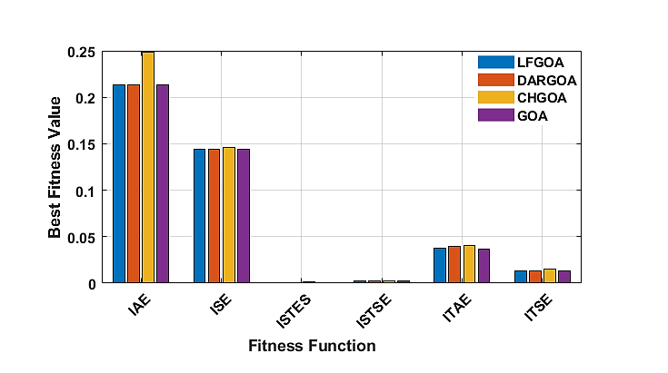
Figure 5. Bar chart illustrating the best fitness values for seven fitness functions obtained using GOA, LFGOA, DARGOA, and CHGOA
- Simulation Results for Linear Desired Input
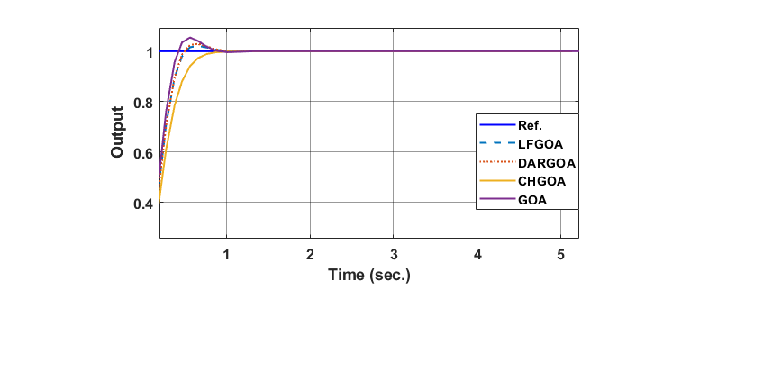
According to ISTES function and linear desired input ( ), the simulation result (output position and control signal) of the controlled MSD based on optimal PID with (GOA, LFGOA, DARGOA, and CHGOA) are shown in Figure 6. These results shows that the actual output of the MSD follow the desired linear input faster with demonstrating stable behavior with variations in settling time, overshoot and error close to zero, where CHGOA exhibited the lowest overshoot.
| 
|
(a) output position (b) Control signal |
Figure 6. Response of MSD system for linear desired input controlled by optimal PID with different GOAs
Table 6 presents the time-domain performance results (rise time ( ), settling time (
 ), overshoot (MOS %), peak value, and best fitness values) obtained from MATLAB/Simulink simulations. These results are evaluated using the six fitness functions (IAE, ISE, ISTES, ISTSE, ITAE, and ITSE) in the simulation environment, each emphasizing different aspects of error minimization and transient performance. The practical time-domain results in Table 6 closely align with the benchmark-based outcomes in Table 2. Specifically, CHGOA consistently achieved top ranks and the lowest best fitness values across multiple CEC2017 functions (F1, F3, F5, F9, F12, F15), which correlates with its ability to eliminate overshoot in ISTES and ITAE, despite a slightly longer . LFGOA and DARGOA also exhibited strong performance in specific benchmark functions (F22 and F23), translating to faster and reduced peak responses in PID control simulations.
Table 6. Comparison of time-response metrics for GOA and modified GOAs across multiple fitness functions
PID based on | Fitness | Rise time () sec. | Settling time () sec. | Peak Value | MOS% | Best Fitness |
LFGOA | IAE | 0.2786 | 0.7515 | 1.1 | 5.18 | 0.21358 |
ISE | 0.2778 | 0.7637 | 1.1 | 5.37 | 0.14376 |
ISTES | 0.3163 | 0.4756 | 1.0 | 1.95 | 0.00013 |
ISTSE | 0.2787 | 0.7502 | 1.1 | 5.16 | 0.00203 |
ITAE | 0.3376 | 0.5145 | 1.0 | 1.42 | 0.03749 |
ITSE | 0.2787 | 0.7501 | 1.1 | 5.16 | 0.01319 |
DARGOA | IAE | 0.2787 | 0.7512 | 1.1 | 5.18 | 0.21358 |
ISE | 0.2778 | 0.7637 | 1.1 | 5.37 | 0.14376 |
ISTES | 0.3161 | 0.7447 | 1.0 | 2.86 | 0.00014 |
ISTSE | 0.2787 | 0.7502 | 1.1 | 5.16 | 0.00203 |
ITAE | 0.3429 | 0.5176 | 1.0 | 1.66 | 0.03944 |
ITSE | 0.2787 | 0.7506 | 1.1 | 5.17 | 0.01319 |
CHGOA | IAE | 0.3401 | 0.7831 | 1.0 | 2.69 | 0.24828 |
ISE | 0.2913 | 0.7822 | 1.0 | 4.48 | 0.14646 |
ISTES | 0.4211 | 0.7057 | 1.0 | 0.0 | 0.00159 |
ISTSE | 0.3276 | 0.495 | 1.0 | 1.56 | 0.00269 |
ITAE | 0.3396 | 0.7952 | 1.0 | 2.8 | 0.04073 |
ITSE | 0.29 | 0.6968 | 1.0 | 3.46 | 0.01524 |
GOA | IAE | 0.2787 | 0.7512 | 1.1 | 5.18 | 0.21358 |
ISE | 0.2778 | 0.764 | 1.1 | 5.38 | 0.14376 |
ISTES | 0.3699 | 0.5753 | 1.0 | 0.5 | 0.00019 |
ISTSE | 0.2787 | 0.751 | 1.1 | 5.18 | 0.00202 |
ITAE | 0.3414 | 0.5284 | 1.0 | 0.92 | 0.03700 |
ITSE | 0.2787 | 0.7496 | 1.1 | 5.16 | 0.01319 |
The results of Figure 6 and Table 6 indicate that LFGOA achieved the best overall performance in the ISTES criterion, with the lowest best fitness value, a short and a fast while maintaining a reduced maximum overshoot. DARGOA produced a similar ISTES performance with nearly identical tr but a slightly higher overshoot. CHGOA, on the other hand, reached a best fitness of 0.001586 with of 0.7057 sec., demonstrated the no overshoot for ISTES, albeit with a longer (0.4211 sec.). The original GOA showed stable performance but was outperformed by some modifications in certain criteria, with its best ISTES value at 0.000194, with 0.3699 sec., and MOS 0.5%. LFGOA and DARGOA exhibited competitive performance in classical error criteria such as IAE and ISE, with nearly identical and times. However, LFGOA consistently provided slightly lower overshoot and better fitness in certain benchmark functions (F22 and F23), making it favorable in scenarios where minimal overshoot and robustness to disturbance are prioritized. Although LFGOA shows slightly better performance in some individual PID metrics (e.g., ISTES), CHGOA consistently outperforms all algorithms across the CEC2017 benchmark functions and maintains a balanced performance in PID metrics, including fitness, rise time, settling time, and MOS%. Therefore, considering both benchmark and PID results, and based on this comprehensive set of performance criteria, CHGOA is regarded as the overall best algorithm.
- Simulation Results for Nonlinear Desired Input
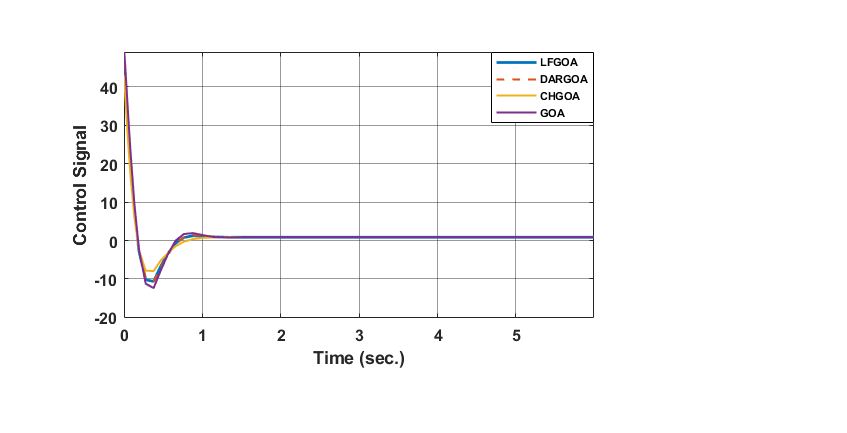
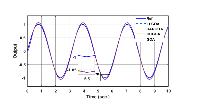
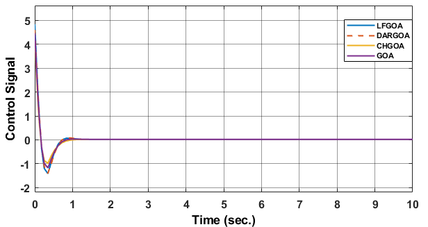
The simulation result (output position and control signal) of the controlled MSD based on optimal PID with (GOA, LFGOA, DARGOA, and CHGOA) for nonlinear ( ) desired input and ISTES function are shown in Figure 7. Table 7 presents the time-domain performance results of the best ISTES fitness function. The results of Figure 7 and Table 7 shows that the performance of the controlled MSD follow the desired nonlinear input faster with error close to zero and minimum ISTES spatially with CHGOA. Overall, the results indicate that while LFGOA and DARGOA are strong choices for conventional performance measures, CHGOA offers the most balanced trade-off between error minimization, convergence rate, and transient performance.
| 
|
(a) output position (b) Control signal
|
Figure 7. Response of MSD system for nonlinear desired input controlled by optimal PID with different GOAs
Table 7. Comparison of time-response fitness functions for GOA and modified GOAs
Optimization | LFGOA | DARGOA | CHGOA | GOA |
ISTES | 18.54 | 20.73 | 14.25 | 17.39 |
- Comparison the results of our optimal PID based on GOAs with results of NPID of Refs. [40][41]
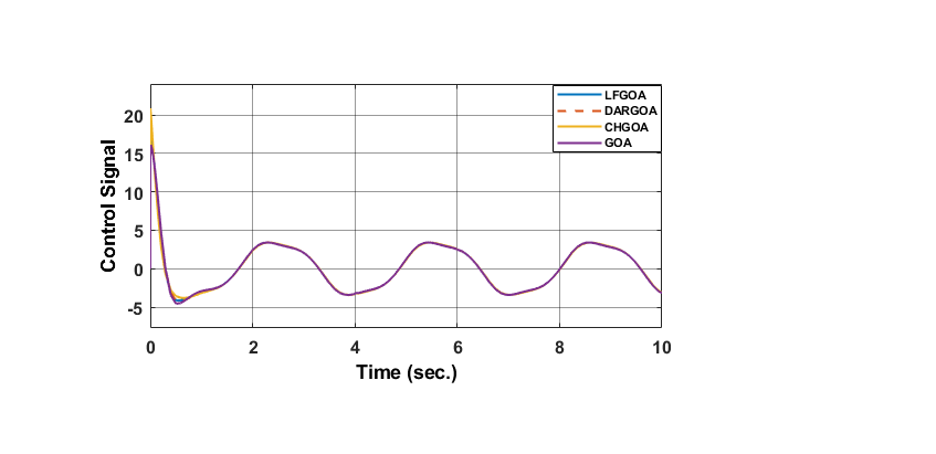
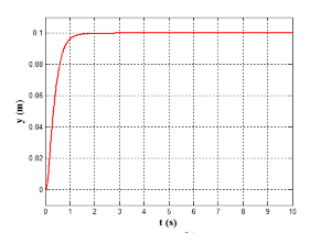
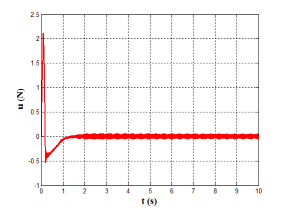
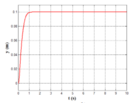
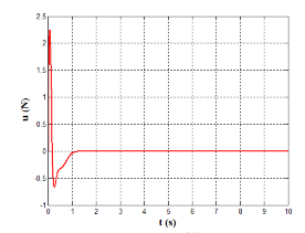
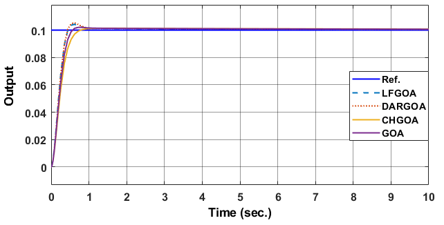
In this subsection, with desired input r(t)= 0.1, the performance of the nonlinear MSD model (Eq. (20) and parameters of Table 3) which is controlled by our suggested optimal PID based on GOAs are also compared with its performance based on two previous proposed modified Nonlinear PID. The first controller is NPID based on modified Han Tracking Differentiator (TD) [41], while the second controller is NPID based on Improved Nonlinear Tracking Differentiator (INTD) with hyperbolic tangent function proposed by Wameedh A. [40]. The simulation results (positions and control signal) for controlled MSD are shown in Figure 8 to Figure10. A comparative performance analysis reveals that the proposed controllers achieve faster settling times compared to both Han and Wameedh methods, even though minor oscillations are observed in certain responses. Nevertheless, all proposed controllers maintain a zero steady-state error, confirming their superior tracking accuracy and stability. Furthermore, the control signal in Han’s and Wameedh’s methods starts approximately from a value of 2, whereas in the proposed methods it starts around 4, indicating a faster transient response. In addition, Han’s controller exhibits noticeable jittering in the control signal, which may induce actuator vibration and undesired fluctuations. In contrast, the suggested optimal PID based on GOAs produce a smoother control signal, ensuring more stable actuation and improved overall system performance.
| 
|
(a) | (b) |
Figure 8. The simulation results of MSD controlled by NPID based on modified Han TD, (a)The control signal u, (b) The plant output y
| 
|
(a) | (b) |
Figure 9. The simulation results of MSD controlled by NPID based on proposed Wameedh INTD, (a) The control signal u (b) The plant output y
| 
|
(a) | (b) |
Figure 10. The simulation results of MSD controlled by optimal PID based on different GOAs, (a) The control signal u (b) The plant output y
- CONCLUSIONS
This paper investigated GOA and three modified GOAs (LFGOA, DARGOA, and CHGOA) to tune the parameters of PID controller which is used to control a SISO nonlinear system. In this paper, a second order MSD is considered as example of SISO nonlinear system. A comprehensive comparison was conducted among the various GOAs. Based on the analysis of best fitness values, rise time, and settling time, the superior performance of CHGOA is evident compared to the other algorithms specifically targeting the reduction of the ISTES objective. Our results confirm that applying the suggested CHGOA achieves better precision tracking and transient stability than LFGOA, DARGOA, and GOA. Therefore, it is recommended to utilize CHGOA for tuning PID, with the ISTES fitness function forming its evaluation basis. Competing algorithms, such as LFGOA and DARGOA, can still enhance system performance in specific scenarios, particularly when minimizing overshoot and ensuring robustness against disturbances are priorities. Future work can expand this research in several directions to further enhance the effectiveness of PID optimization algorithms for the second order and higher order nonlinear SISO system and the potential directions can be include:
- Developing hybrid algorithms combining CHGOA with specific techniques like PSO or AOA, integrating advanced strategies such as Levy Flight or Opposition-based Learning to improve convergence speed and solution accuracy.
- Exploring more advanced controller types, such as FOPID or Fuzzy PID, and comparing them with conventional controllers to enhance real-time control of nonlinear systems.
- Adopting multi-objective optimization to minimize multiple performance metrics simultaneously, such as settling error, rise time, and overshoot, while providing Pareto-optimal solutions
DECLARATION
Author contribution
Aliaa A. Flaih: Original draft preparation, Formal analysis, Investigation, Software; Ekhlas H. Karam: Manuscript writing and review, Validation of results, Investigation, Yousra A. Mohammed: Investigation, Formal analysis and Validation of results.
Conflict of interest
The authors have no conflict of interest to declare.
Funding
The authors received no specific funding for this work.
Acknowledgement
We would like to express our deep appreciation to whom giving us much time, effort, and best guidance throughout the work.
REFERENCES
- H. Yu, Z. Hou and X. Yu, "A Controller-Dynamic-Linearization-Based Model Predictive Control Approach for SISO Discrete-time Nonlinear Systems," 2019 12th Asian Control Conference (ASCC), pp. 1054-1059, 2019, https://ieeexplore.ieee.org/abstract/document/8765146.
- H. Boumaza and K. Belarbi, “Optimal model predictive control solution approximation using Takagi Sugeno for linear and a class of nonlinear systems,” Int. J. Dyn. Control, vol. 10, no. 4, pp. 1265–1278, 2022, https://doi.org/10.1007/s40435-021-00875-4.
- Z. Wang and R. M. Jungers, “Immersion-based model predictive control of constrained nonlinear systems: Polyflow approximation,” 2021 Eur. Control Conf. ECC 2021, no. 0, pp. 1099–1104, 2021, https://doi.org/10.23919/ECC54610.2021.9655233.
- D. R. Raghavendra, “Control of SISO EH Servo Systems,” in Electrohydraulic Servo Systems: Applications, Design and Control, pp. 111–171, 2023, https://doi.org/10.1007/978-981-19-8065-7_5.
- P. Razzaghi, E. Al Khatib, and Y. Hurmuzlu, “Robust Quadratic Gaussian Control of Continuous-time Nonlinear Systems,” arXiv preprint arXiv:1912.06717, 2019, https://doi.org/10.48550/arXiv.1912.06717.
- B. N. Getu, “Modelling and Analysis of a Nonlinear System using Simulink,” in 2019 International Conference on Electrical and Computing Technologies and Applications (ICECTA), pp. 1–4, 2019, https://doi.org/10.1109/ICECTA48151.2019.8959725.
- A. Lozynskyy, L. Kasha, S. Pakizh, and R. Sadovskyi, “Synthesis of PI- and PID-Regulators in Control Systems Derived by the Feedback Linearization Method,” Energy Eng. Control Syst., vol. 10, no. 2, pp. 120–130, 2024, https://doi.org/10.23939/jeecs2024.02.120.
- E. H. Karam, N. A. Al-Awad, and N. S. Abdul-Jaleel, “Design nonlinear model reference with fuzzy controller for nonlinear SISO second order systems,” Int. J. Electr. Comput. Eng., vol. 9, no. 4, pp. 2491–2502, 2019, https://doi.org/10.11591/ijece.v9i4.pp2491-2402.
- F. Zhang, J. Hua, and Y. Li, “Indirect Adaptive Fuzzy Control of SISO Nonlinear Systems With Input–Output Nonlinear Relationship,” IEEE Trans. Fuzzy Syst., vol. 26, no. 5, pp. 2699–2708, 2018, https://doi.org/10.1109/TFUZZ.2018.2800714.
- S. Chen, W. Huang, and Q. Liu, “A New Adaptive Robust Sliding Mode Control Approach for Nonlinear Singular Fractional-Order Systems,” Fractal Fract., vol. 6, no. 5, pp. 1–19, 2022, https://doi.org/10.3390/fractalfract6050253.
- B. Li, J. Zhu, R. Zhou, and G. Wen, “Adaptive Neural Network Sliding Mode Control for a Class of SISO Nonlinear Systems,” Mathematics, vol. 10, no. 7, pp. 1–12, 2022, https://doi.org/10.3390/math10071182.
- C. Yue, H. Chen, L. Qian, and J. Kong, “Adaptive sliding-mode tracking control for an uncertain nonlinear SISO servo system with a disturbance observer,” J. Shanghai Jiaotong Univ., vol. 23, no. 3, pp. 376–383, 2018, https://doi.org/10.1007/s12204-018-1953-6.
- P. Kumar, S. Nema, and P. K. Padhy, “PID controller for nonlinear system using cuckoo optimization,” 2014 Int. Conf. Control. Instrumentation, Commun. Comput. Technol. ICCICCT 2014, pp. 711–716, 2014, https://doi.org/10.1109/ICCICCT.2014.6993052.
- H. I. Ali, H. M. Jassim, and A. F. Hasan, “Optimal Nonlinear Model Reference Controller Design for Ball and Plate System,” Arab. J. Sci. Eng., vol. 44, no. 8, pp. 6757–6768, 2019, https://doi.org/10.1007/s13369-018-3616-1.
- J. Cheng and Y. Xiong, “Multi-strategy adaptive cuckoo search algorithm for numerical optimization,” Artif. Intell. Rev., vol. 56, no. 3, pp. 2031–2055, 2023, https://doi.org/10.1007/s10462-022-10222-4.
- L. Velasco, H. Guerrero, and A. Hospitaler, “A Literature Review and Critical Analysis of Metaheuristics Recently Developed,” Arch. Comput. Methods Eng., vol. 31, no. 1, pp. 125–146, 2024, https://doi.org/10.1007/s11831-023-09975-0.
- E. H. Houssein, M. K. Saeed, G. Hu, and M. M. Al-Sayed, Metaheuristics for Solving Global and Engineering Optimization Problems: Review, Applications, Open Issues and Challenges, vol. 31, no. 8, 2024. https://doi.org/10.1007/s11831-024-10168-6.
- V. Srivastava, S. Srivastava, G. Chaudhary, and X. P. Blanco Valencia, “Performance improvement and Lyapunov stability analysis of nonlinear systems using hybrid optimization techniques,” Expert Syst., vol. 41, no. 6, p. e13140, 2024, https://doi.org/10.1111/exsy.13140.
- V. Kaliappan, “Nonlinear PID controller parameter optimization using enhanced genetic algorithm for nonlinear control system,” J. Control Eng. Appl. Informatics, vol. 18, no. 2, pp. 3–10, 2016, https://ceai.srait.ro/index.php?journal=ceai&page=article&op=view&path%5B%5D=2891&path%5B%5D=0.
- Z. Chu, Q. Guo, and C. Wang, “The PID Control Algorithm based on Whale Optimization Algorithm Optimized BP Neural Network,” in 2023 IEEE 7th Information Technology and Mechatronics Engineering Conference (ITOEC), vol. 7, pp. 2450–2453, 2023, https://doi.org/10.1109/ITOEC57671.2023.10291531.
- D. Nasri and D. Mokeddem, “Optimisation of multi-objective problems using an efficient Levy flight grasshopper algorithm,” Int. J. High Perform. Syst. Archit., vol. 11, no. 1, pp. 26–35, 2022, https://doi.org/10.1504/IJHPSA.2022.121901.
- L. Wu, J. Wu, and T. Wang, “Enhancing grasshopper optimization algorithm (GOA) with levy flight for engineering applications,” Scientific reports, vol. 13, no. 1, 2023. https://doi.org/10.1038/s41598-022-27144-4.
- Y. Zou, B. Xiao, J. Qian, and Z. Xiao, “Design of Intelligent Nonlinear H2/H∞ Robust Control Strategy of Diesel Generator-Based CPSOGSA Optimization Algorithm,” Processes, vol. 11, no. 7, pp. 1–28, 2023, https://doi.org/10.3390/pr11071867.
- Y. Deng, W. Song, S. Yin, M. Zhong, K. Yang and X. Feng, "A Model Predictive Control Scheme Without Current Sensor of Dual Active Bridge DC–DC Converters: Improving Dynamic Performance and Reducing Hardware Cost," in IEEE Transactions on Transportation Electrification, vol. 9, no. 2, pp. 2916-2928, 2023, https://doi.org/10.1109/TTE.2022.3229076.
- S. Saremi, S. Mirjalili, and A. Lewis, “Grasshopper Optimisation Algorithm: Theory and application,” Adv. Eng. Softw., vol. 105, pp. 30–47, 2017, https://doi.org/10.1016/j.advengsoft.2017.01.004.
- A. A. Ewees, M. A. Elaziz, Z. Alameer, H. Ye, and Z. Jianhua, “Improving multilayer perceptron neural network using chaotic grasshopper optimization algorithm to forecast iron ore price volatility,” Resour. Policy, vol. 65, p. 101555, 2020, https://doi.org/10.1016/j.resourpol.2019.101555.
- S. Jain and K. K. Bharti, “Chaos inspired Particle Swarm Optimization with Levy Flight for Genome Sequence Assembly,” arXiv preprint arXiv:2110.10623, 2021, https://doi.org/10.48550/arXiv.2110.10623.
- S. Mirjalili, “Dragonfly algorithm: a new meta-heuristic optimization technique for solving single-objective, discrete, and multi-objective problems,” Neural Comput. Appl., vol. 27, no. 4, pp. 1053–1073, 2016, https://doi.org/10.1007/s00521-015-1920-1.
- Y. Meraihi, A. B. Gabis, S. Mirjalili, and A. Ramdane-Cherif, “Grasshopper optimization algorithm: theory, variants, and applications,” Ieee Access, vol. 9, pp. 50001–50024, 2021, https://doi.org/10.1109/ACCESS.2021.3067597.
- G. S. Kumar, G. Sahu, and M. Mathur, “A modified grasshopper optimization algorithm based on levy flight for cluster head selection in wireless sensor networks,” Int. J. Adv. Technol. Eng. Explor., vol. 9, no. 97, p. 1846, 2022, https://doi.org/10.19101/IJATEE.2021.875883.
- W. Liu, W. Yan, T. Li, G. Han, and T. Ren, “A Multi-strategy Improved Grasshopper Optimization Algorithm for Solving Global Optimization and Engineering Problems,” Int. J. Comput. Intell. Syst., vol. 17, no. 1, 2024, https://doi.org/10.1007/s44196-024-00578-6.
- S. Arora and P. Anand, “Chaotic grasshopper optimization algorithm for global optimization,” Neural Comput. Appl., vol. 31, no. 8, pp. 4385–4405, 2019, https://doi.org/10.1007/s00521-018-3343-2.
- Y. A. N. Yan, M. A. Hongzhong, and L. I. Zhendong, “An Improved Grasshopper Optimization Algorithm for Global Optimization,” Chinese J. Electron., vol. 30, no. 3, pp. 451–459, 2021, https://doi.org/10.1049/cje.2021.03.008.
- M. Sallam, I. Saif, Z. Saeed, and M. Fanni, “Lyapunov-based control of a teleoperation system in presence of time delay,” in International Conference on Advanced Intelligent Systems and Informatics, pp. 759–768, 2020, https://doi.org/10.1007/978-3-030-58669-0_67.
- W. Aribowo et al., “Sand cat swarm optimization for controlling PID in DC motor,” Telkomnika (Telecommunication Comput. Electron. Control., vol. 22, no. 2, pp. 462–470, 2024, https://doi.org/10.12928/TELKOMNIKA.v22i2.25630.
- A. M. Abushanab, H. M. Hasanien, and R. M. Sharkawy, “Frequency control of interconnected power system using dandelion optimization algorithm,” in 2024 6th International youth conference on radio electronics, electrical and power engineering (REEPE), pp. 1–7, 2024, https://doi.org/10.1109/REEPE60449.2024.10479799.
- A. M. Abushanab, H. M. Hasanien, and R. M. Sharkawy, “Frequency Control of Interconnected Power System Utilizing Novel Optimization Approaches,” in 2024 FORTEI-International Conference on Electrical Engineering (FORTEI-ICEE), pp. 24–29, 2024, https://doi.org/10.1109/FORTEI-ICEE64706.2024.10824329.
- S. Mirjalili, S. M. Mirjalili, and A. Lewis, “Grey Wolf Optimizer,” Adv. Eng. Softw., vol. 69, pp. 46–61, 2014, https://doi.org/10.1016/j.advengsoft.2013.12.007.
- A. Mulyadi, M. Z. R. Amin, and M. K. Anam, “Control Mass-Spring-Damper Based on Tuning Trade-off PID Controller,” J. Ecotipe (Electronic, Control. Telecommun. Information, Power Eng., vol. 10, no. 1, pp. 52–60, 2023, https://doi.org/10.33019/jurnalecotipe.v0i0.3723.
- I. Kasim and W. Riyadh, “On the Improved Nonlinear Tracking Differentiator based Nonlinear PID Controller Design,” Int. J. Adv. Comput. Sci. Appl., vol. 7, no. 10, 2016, https://doi.org/10.14569/ijacsa.2016.071032.
- J. Wei and Z. Gao, “Design and analysis on fractional-order tracking differentiator,” in The 27th Chinese Control and Decision Conference (2015 CCDC), pp. 6128–6132, 2015, https://doi.org/10.1109/CCDC.2015.7161912.
Appendix A
Table A1. Unimodal benchmark functions.
Function | Range | D |
|
 (y)= (y)=
| [-100,100] | 30 | 0 |
 (y)= (y)=
| [-10,100] | 30 | 0 |
 (y)= (y)=
| [-100,100] | 30 | 0 |
 (y)= (y)=
| [-100,100] | 30 | 0 |
 (y)= (y)=
| [-30,30] | 30 | 0 |
 (y)= (y)=
| [-100,100] | 30 | 0 |
 (y)= (y)=
| [-1.28,1.28] | 30 | 0 |
Table A2. Multimodal benchmark functions
Function | Range | D |
|
 (y)= (y)=
| [-500,500] | 30 | -12569.5 |
 (y)= (y)=
| [-5.12,5.12] | 30 | 0 |
 (y)= (y)=

| [-32,32] | 30 | 0 |
 (y)= (y)=
| [-600,600] | 30 | 0 |
 (y)= (y)=


| [-50,50] | 30 | 0 |
 (y)= (y)=
| [-50,50] | 30 | 0 |
Table A3. Fixed-dimension multimodal benchmark functions
Function | Range | D |
|
 (y)= (y)=
| [-65,65] | 2 | 1 |
 (y)= (y)=
| [-5,5] | 4 | 0.00030 |
 (y)= (y)=
| [-5,5] | 2 | -1.0316 |
 (y)= (y)=
| [-5,5] | 2 | 0.398 |
 (y)= (y)=
| [-2,2] | 2 | 3 |
 (y)= (y)=
| [1,3] | 3 | -3.86 |
 (y)= (y)=
| [0,1] | 6 | -3.32 |
 (y)= (y)=
| [0,10] | 4 | -10.1532 |
 (y)= (y)=
| [0,10] | 4 | -10.4028 |
 (y)= (y)=
| [0,10] | 4 | -10.5363 |
AUTHOR BIOGRAPHY

| Aliaa A. Flaih She received her B.Sc. and M.Sc. degrees in Computer Engineering from Al-Mustansiriyah University, Baghdad, Iraq, where she is currently working as a faculty member. Her research interests include machine learning, artificial intelligence systems, image processing, and robotics. She can be contacted at Email: aliaa.adnan.f@uomustansiriyah.edu.iq https://orcid.org/0009-0003-3869-6584 |
|
|

| Ekhlas H. Karam completed her M.Sc. in control engineering, University of Technology\Control and Systems Engineering Department, Baghdad, Iraq (2001), and Ph.D. in Mechatronics Engineering, University of Technology\Control and Systems Engineering Department, Baghdad, Iraq (2007). Currently, she is working as a professor in the Computer Department, Faculty of Engineering, Al-Mustansiriyah University. Her research interests are in robotic and automation systems, adaptive and robust controller designs, optimization methods, and Artificial intelligence systems. Email: ek_karam@uomustansiriyah.edu.iq https://orcid.org/0000-0002-9039-2030 |
|
|

| Yousra A. Mohammed is a lecturer at the Communication Engineering Department, Technology University, Baghdad, Iraq since 2005. She received her B.Sc. in Electronic and Communication Engineering from Technology University/Baghdad, Iraq in 1992 and her M.Sc. degree in Computer Engineering from Technology University/Baghdad in 2004. Her research interests include Control Systems, Encryption and Decryption Algorithms, Artificial intelligence systems and IoT. Email: yousra.a.mohammed@uotechnology.edu.iq https://orcid.org/0000-0002-6432-0754 |
Aliaa A. Flaih (Optimal PID Controller Based on Different Modified Grasshopper Optimization Algorithm for Nonlinear Single-Input Single-Output System)