ISSN: 2685-9572 Buletin Ilmiah Sarjana Teknik Elektro
Vol. 7, No. 3, September 2025, pp. 625-640
Bayesian-Optimized MLP-LSTM-CNN for Multi-Year Day-Ahead Electric Load Forecasting
Tuan Anh Nguyen, Nguyen Trung Dung
FEET, Industrial University of Ho Chi Minh City (IUH), Ho Chi Minh City, Viet Nam
ARTICLE INFORMATION |
| ABSTRACT |
Article History: Received 26 July 2025 Revised 23 September 2025 Accepted 09 October 2025 |
| 
Accurate long-term electric load forecasting—multi-year, day-ahead peak-load prediction—is critical for planning, operations, and policy. While traditional statistical and shallow machine-learning methods often struggle with nonlinear and multi-scale temporal patterns, deep learning offers promising alternatives. This study conducts a systematic, controlled comparison of three architectures—Multilayer Perceptron (MLP), Convolutional Neural Network (CNN), and Long Short-Term Memory (LSTM)—within a unified Bayesian hyperparameter optimization protocol using daily peak-load data from the New South Wales (NSW) electricity market, 2015–2021, with a 365-day look-back window. Under identical data splits, objective, and search procedures, CNN delivers the best accuracy across all metrics (MAE = 699, MSE = 791,838, RMSE = 890, MAPE = 7.53%), MLP performs slightly worse, and LSTM yields the most significant errors alongside the most extended runtime. These results indicate that, under consistent tuning and a one-year context window, CNN captures local variations more effectively than the recurrent alternative in this setting. The research contribution of this study is a fair, empirical benchmark of widely used deep models (MLP, CNN, LSTM) for multi-year, day-ahead peak-load forecasting under a single Bayesian optimization framework, offering practical guidance for model selection. Reproducibility is facilitated by fixed random seeds and comprehensive configuration/trace logging. Limitations include an intentionally univariate design (no exogenous variables), a focus on learned architectures rather than naïve baselines, and the absence of uncertainty quantification; future work will extend to multivariate inputs (e.g., weather and calendar effects), hybrid CNN–LSTM and Transformer-based models, and broader baseline and robustness evaluations. |
Keywords: Electric Load Forecasting; Time-Series Forecasting; Deep Learning; Bayesian Optimization; MLP; LSTM; CNN |
Corresponding Author: Nguyen Trung Dung,
FEET, Industrial University of Ho Chi Minh City,
Ho Chi Minh City, Viet Nam
Email: nguyentrungdung@iuh.edu.vn |
This work is licensed under a Creative Commons Attribution-Share Alike 4.0 
|
Document Citation: T. A. Nguyen and N. T. Dung, “Bayesian-Optimized MLP-LSTM-CNN for Multi-Year Day-Ahead Electric Load Forecasting,” Buletin Ilmiah Sarjana Teknik Elektro, vol. 7, no. 3, pp. 625-640, 2025, DOI: 10.12928/biste.v7i3.14345. |
- INTRODUCTION
Long-term electric load forecasting is crucial in power system planning, generation scheduling, and stable grid operation. In this study, “long-term” refers to multi-year, day-ahead peak-load forecasting using daily data, which directly supports capacity planning, asset investment, tariff design, and policy decisions. Accurate long-term forecasts enable utilities to optimize resource allocation and maintain system reliability while minimizing operational costs and the risk of outages. We focus on New South Wales (NSW), Australia, from 2015 to 2021, which captures typical seasonality and pandemic-related anomalies, providing a challenging and representative evaluation setting. Historically, traditional statistical and econometric models such as regression [1]–[5], ARIMA (Autoregressive Integrated Moving Average) [6]–[10], and exponential smoothing [11]–[14] have been widely applied in load forecasting due to their simplicity, ease of implementation, and effectiveness when data exhibit linear and stable patterns. However, these approaches face significant limitations in modeling complex nonlinear relationships and tend to lose accuracy when the data are highly volatile because of seasonal factors, weather conditions, or sudden demand shocks. To address these limitations, machine learning methods such as Support Vector Regression (SVR) [15]–[18], Random Forests [19]–[20], and Extreme Gradient Boosting (XGBoost) [21]–[27] have been introduced, offering improved capability in capturing nonlinearities, handling large datasets, and achieving higher accuracy than traditional models. Nevertheless, these methods rely heavily on manual feature engineering, are prone to overfitting without careful tuning, and are less effective at fully capturing the temporal dependencies inherent in electricity load data.
The emergence of deep learning has opened a new direction for load forecasting, overcoming many limitations of traditional and machine-learning approaches. Models such as Convolutional Neural Networks (CNNs) [28]–[37], Long Short-Term Memory (LSTM) networks [38]–[43], and Multilayer Perceptrons (MLPs) [44]–[49] enable automatic feature extraction, represent complex nonlinear dependencies, and capture temporal dynamics with limited manual preprocessing. The Transformer architecture [50]–[56], originally developed for natural language processing, has also been applied to time-series forecasting via attention mechanisms that capture both short- and long-term dependencies. However, to establish a transparent and interpretable baseline across canonical DL architectures, this study focuses on MLP, CNN, and LSTM; Transformer-based models are left to future work due to their substantially higher design complexity and computational cost. Despite this progress, two gaps remain for long-term horizons. First, prior studies rarely provide an apples-to-apples comparison of MLP, CNN, and LSTM under a unified hyperparameter optimization protocol, making it challenging to attribute performance differences to architectures rather than tuning choices. Second, evidence is limited regarding which architecture is most suitable when models are tuned consistently and evaluated on the same long-horizon data and metrics. Forecasting accuracy and robustness depend on architectural design and hyperparameters (e.g., number of layers/neurons, learning rate, batch size, regularization). Regardless of architectural advances, the performance of deep models hinges on proper hyperparameter configuration. While grid search, random search, and metaheuristics have been applied, they can be computationally expensive and inefficient in large search spaces. In this context, Bayesian optimization [57]–[63] offers a practical balance between exploration and exploitation, typically requiring fewer model evaluations to approach optimal configurations.
This study addresses the aforementioned gaps by conducting a controlled comparative evaluation of MLP, CNN, and LSTM for long-term (multi-year, day-ahead peak-load forecasting using daily data) electric load forecasting under a unified Bayesian hyperparameter optimization framework. We standardize data splits, the objective (validation MAPE), and model-specific search spaces across all architectures to ensure fair comparability. The research contribution is threefold: A systematic, controlled comparison of MLP, CNN, and LSTM for long-term, day-ahead peak-load forecasting using daily data under a unified Bayesian optimization framework; Empirical evidence showing that CNN achieves the best overall accuracy across MAE, MSE, RMSE, and MAPE, with MLP close behind and LSTM underperforming both in accuracy and runtime; Practical guidance for selecting DL architectures in long-term planning, clarifying the trade-offs between accuracy and computational cost. Scope and research focus. We aim to quantify how Bayesian hyperparameter optimization affects different learned architectures under an identical search budget. Accordingly, we emphasize like-for-like comparisons among MLP, CNN, and LSTM. While simple seasonal/persistence baselines provide proper context, a comprehensive baseline survey would broaden the scope beyond our optimization-centric research questions and is therefore deferred to future work; this is noted again in the limitations.
- THEORETICAL BACKGROUND
- MLP – Multilayer Perceptron
The Multi-Layer Perceptron (MLP) is a subclass of artificial neural networks widely used for classification and regression tasks. As a Deep Neural Network (DNN) family member, MLPs can approximate complex nonlinear relationships, making them suitable for high-dimensional and nonlinear problems. An MLP consists of three main components: an Input layer receiving raw features; Hidden layers extracting hierarchical patterns through weighted linear combinations and nonlinear activation functions; and an Output layer that produces the final prediction (a class label for classification or a continuous value for regression). The learning process of an MLP includes forward propagation and backpropagation. In forward propagation, inputs are transformed layer by layer through linear operations and activation functions. Backpropagation then adjusts the weights and biases using gradients of the loss function to minimize prediction errors. Where,  is the linear combination between the pre-layer output and weights, plus bias.
  is the weighted matrix between class -1 and class
  .
.  is the output of class -1 .
  : Is the bias of the class .
  is the output of the second class, which is the result after applying the trigger function
 .
.  is the trigger function.
  is the predicted output value.
  is the actual value.
  is the derivative of the loss function L for class output .
  is the number of samples in the training dataset. Gradient for calculation via trigger function .
  is the gradient of the loss function for pure input . is the gradient of the loss function to the output of the class . is the weighted matrix in the second class .
  is the learning rate.
  is the derivative (gradient) of the loss function L by weight . Is the speed of learning. is the bias of the class, making the model more flexible when learning.
  : The derivative of the loss function L for the bias in the class .
| 
| (1) |
| 
| (2) |
| 
| (3) |
| 
| (4) |
| 
| (5) |
| 
| (6) |
| 
| (7) |
| 
| (8) |
| 
| (9) |
| 
| (10) |
| 
| (11) |
| 
| (12) |
| 
| (13) |
- LSTM – Long Short-Term Memory
Long Short-Term Memory (LSTM) networks are specialized Recurrent Neural Networks (RNNs) designed to capture long-term dependencies in sequential data. Unlike conventional RNNs, which often suffer from vanishing or exploding gradients when trained on long sequences, LSTM networks employ a memory cell and a system of gates—input, forget, and output—that regulate the flow of information. This gating mechanism allows the network to retain valuable information and selectively discard irrelevant details over time. An LSTM cell is composed of four key elements: a memory cell that stores information across multiple time steps, an input gate that controls the incorporation of new information, a forget gate that decides which data to discard, and an output gate that regulates the information passed to the next layer. These gates use nonlinear activation functions, typically the sigmoid and hyperbolic tangent (tanh), to determine how much information flows through the cell at each step.
This structure makes LSTM networks highly effective for modeling nonlinear relationships and temporal dependencies in time-series data, including electricity load forecasting. They can learn from historical consumption patterns, seasonal fluctuations, and external variations to predict future demand. The selective memory mechanism enables LSTM to retain critical historical context while filtering noise, often resulting in superior accuracy compared to traditional RNNs. However, the performance of LSTM is sensitive to hyperparameters such as the number of layers, memory units, learning rate, batch size, and dropout rate. Poorly tuned configurations may lead to underfitting, overfitting, or slow convergence, highlighting the necessity of systematic hyperparameter optimization to fully exploit the forecasting capabilities of LSTM models. The internal operations of an LSTM cell can be mathematically formulated as follows, where the gating mechanisms regulate the flow of information over time:
At time t, the input variable is denoted as  . The symbols
  represent the weight matrices, where it corresponds to the input gate, and
  denote the forget gate, output gate, and cell state, respectively. The sigmoid activation function is denoted by σ, while
  represents the hidden state output at time t in vector form. Additionally,
  are the bias terms associated with each gate in the LSTM architecture.
- CNNs - Convolutional Neural Network
Convolutional Neural Networks (CNNs) are robust deep learning architectures that process grid-structured data, such as images and one-dimensional time series. Initially developed for computer vision tasks like face recognition, object classification, and localization, CNNs have been successfully adapted for short-term load forecasting (STLF). A typical CNN model consists of four main components: Convolutional layers, which extract local features using learnable filters. Activation functions: introduce nonlinearity to enhance representational capacity. Pooling layers: reduce dimensionality and computational complexity. Fully connected layers: integrate extracted features for the final prediction. In time-series forecasting, 1-D CNNs are applied by sliding kernels along the temporal dimension to capture sequential patterns such as daily or seasonal load curves. CNNs are advantageous compared to recurrent models due to faster training, parallelization capability, and effective performance even with limited historical data. However, their effectiveness depends on appropriate hyperparameter selection (e.g., number of layers, filters, kernel size, learning rate, batch size, and epochs).
Where,  is the value at position
  in the feature map. size
  filter of size .
  is the represents the corresponding region in the input image.
  is the input of the activation function, which selects the better value between
  and . If is less than , the output will be ; if is greater than , the output will remain . The ReLU function enhances the neural network’s ability to learn nonlinear features while reducing the vanishing gradient problem, making the model more efficient during training.
  ) is a small region in the feature map. is the input from the previous layer.
  is the weighted matrix, and b is the bias vector.
- Bayesian Hyperparameter Optimization
Hyperparameter optimization improves deep learning models' performance and generalization ability. Unlike model parameters learned during training, hyperparameters such as the number of layers, hidden units, learning rate, batch size, and dropout rate must be predefined. Poorly chosen hyperparameters may lead to underfitting, overfitting, or unstable convergence, reducing forecasting accuracy. Traditional search methods, such as grid search and random search, are limited in efficiency because they require extensive evaluations over large search spaces, making them computationally expensive. Bayesian optimization offers an efficient alternative by treating hyperparameter tuning as a black-box optimization problem. Instead of exhaustively searching the space, Bayesian methods build a probabilistic surrogate model (commonly Gaussian Processes or Tree-structured Parzen Estimators) to approximate the relationship between hyperparameters and validation performance. At each iteration, the surrogate model predicts promising hyperparameter configurations, while an acquisition function balances exploration of untested regions and exploitation of known good areas. This approach allows Bayesian optimization to converge faster to near-optimal solutions with fewer evaluations than conventional methods. In load forecasting, Bayesian optimization is applied to systematically tune the hyperparameters of MLP, CNN, and LSTM models. The objective is to minimize forecasting error, measured by metrics such as Mean Absolute Error (MAE), Root Mean Square Error (RMSE), and Mean Absolute Percentage Error (MAPE). By integrating Bayesian optimization into the training pipeline, this study ensures fair comparison among models and highlights the impact of hyperparameter tuning on improving predictive accuracy and model reliability.
- PROPOSED METHOD
- Model Architectures MLP
The Multilayer Perceptron (MLP) model was implemented as a baseline deep learning architecture for long-term electric load forecasting. The network consists of four fully connected hidden layers, where the number of neurons in each layer is treated as a tunable hyperparameter. Specifically, the search space included {16, 32, 64, 128} neurons per hidden layer, allowing the architecture to adaptively capture nonlinear dependencies in the data. All hidden layers used the Rectified Linear Unit (ReLU) activation function to improve convergence speed and mitigate the vanishing gradient problem. The output layer contained a single linear unit to generate continuous load forecasts. The Adam optimizer optimized the model with a fixed learning rate of 0.001. Two alternative loss functions—Mean Squared Error (MSE) and Mean Absolute Error (MAE)—were incorporated into the hyperparameter search to ensure fairness in evaluation. In addition, the batch size was selected from {16, 32, 64}, and the number of training epochs ranged from 50 to 250. Bayesian Optimization with Gaussian Process priors (BayesSearchCV) was employed to explore the hyperparameter space efficiently. A three-fold cross-validation scheme was used, with the Mean Absolute Percentage Error (MAPE) as the objective scoring metric. Each configuration was evaluated across folds to compute the average validation error. The best-performing set of hyperparameters was selected based on the lowest cross-validated MAPE, ensuring robust generalization to unseen data. The complete training and hyperparameter optimization process was timed to record computational cost. This procedure provides predictive accuracy and a fair basis for comparing the MLP against other CNN and LSTM architectures under a consistent evaluation framework.
- Model Architectures LSTM
The Long Short-Term Memory (LSTM) network was adopted to capture long-range temporal dependencies inherent in electric load data. The architecture consisted of four stacked LSTM layers, each parameterized by a tunable number of units selected from {16, 32, 64, 128}. All hidden layers employed the Rectified Linear Unit (ReLU) activation function to enhance non-linearity and mitigate vanishing gradient issues. Dropout with a fixed rate of 0.2 was applied after each recurrent layer to prevent overfitting. The final layer of the model was a fully connected dense layer with a single linear neuron, producing the load forecast. The optimizer used was Adam with a learning rate of 0.001. Mean Squared Error (MSE) and Mean Absolute Error (MAE) were included as candidate loss functions in the hyperparameter search to ensure a fair comparison across architectures. Additional hyperparameters considered included batch size {16, 32, 64} and epochs {50, 100, 150, 200, 250}. The model was trained using Bayesian Search. Each candidate configuration was evaluated using three-fold time series cross-validation, and the mean Mean Absolute Percentage Error (MAPE) was employed as the optimization criterion. Early stopping was applied to reduce overfitting and shorten training time. The optimization process yielded the best-performing LSTM configuration, which was stored in JSON and CSV formats for reproducibility and further analysis. This systematic tuning ensures that the LSTM results are directly comparable with those of the MLP and CNN architectures under the same experimental framework.
- Model Architectures CNN
The Convolutional Neural Network (CNN) architecture was designed to capture local temporal patterns in the load data through convolutional feature extraction. The model consists of four one-dimensional convolutional layers, each parameterized by a tunable number of filters selected from {16, 32, 64, 128}. All convolutional layers employed a kernel size of 3 with “same” padding to preserve the input dimensionality, and used the Rectified Linear Unit (ReLU) activation function for non-linearity. Following the convolutional blocks, the extracted features were flattened and passed through a fully connected dense layer with 64 neurons and ReLU activation. A dropout layer with a fixed rate 0.2 was applied to mitigate overfitting before the output stage. The final output layer was a single linear neuron, producing continuous electric load forecasts. The network was optimized using the Adam optimizer with a learning rate 0.001. Mean Squared Error (MSE) and Mean Absolute Error (MAE) loss functions were incorporated into the hyperparameter search to maintain fairness across models. The batch size was also selected from {16, 32, 64}, and the number of epochs ranged between 50 and 250. For hyperparameter optimization, Bayesian Optimization was employed through BayesSearch with 20 iterations. A three-fold cross-validation scheme was applied, and the objective metric was the Mean Absolute Percentage Error (MAPE). Each candidate configuration was evaluated across folds, and the mean validation MAPE was used to guide the optimization. The total training time for the search was recorded to quantify computational cost. The optimal hyperparameters identified by this process represent the most effective CNN configuration under the evaluation framework, allowing for a fair performance comparison with MLP and LSTM architectures.
- Bayesian Hyperparameter Optimization and Evaluation Protocol
To enable a fair and systematic comparison, the hyperparameters of the MLP, CNN, and LSTM models were optimized with BayesSearchCV (scikit-optimize). The Bayesian procedure employs a Gaussian-process surrogate and an exploration–exploitation acquisition rule to traverse the search space efficiently. The series was first split chronologically into 80% training and 20% hold-out test (shuffle = False). Within the training 80%, each candidate configuration was evaluated via three-fold time-series cross-validation under an expanding-window protocol (no shuffling; a temporal gap was used to mitigate leakage). The objective minimized during model selection was the mean cross-validated MAPE (%), implemented as scoring='neg_mean_absolute_percentage_error'. After model selection, the best configuration for each architecture was retrained on the 80% training subset and assessed on the 20% hold-out test using MAE, MSE, RMSE, and MAPE. Training employed early stopping (monitoring validation loss, patience = 10, restoring best weights) to reduce overfitting and shorten evaluation time. The search budget was set to 20 trials per architecture to balance solution quality and computational cost. No feature scaling or normalization was applied; Peak Load remains in MW throughout preprocessing and modeling. An additional advantage of BayesSearchCV is sample efficiency. By fitting a Gaussian-process surrogate and using an uncertainty-aware acquisition rule (e.g., expected improvement or lower confidence bound), it concentrates evaluations on promising regions of the search space and often finds strong configurations under a small budget. The method naturally supports mixed hyperparameter types (continuous, integer, categorical), integrates cleanly with time-series cross-validation, and is robust to noisy fold estimates by modeling uncertainty rather than relying on single point evaluations—thereby lowering computational cost and reducing the risk of overfitting to a single split. Environment and reproducibility. Experiments were conducted on Google Colab (high-performance CPUs and ample memory) using Python 3.10 and TensorFlow 2.12. Random seeds were fixed for all runs, and complete optimization traces (hyperparameters, fold-wise scores, and early-stopping epochs) were logged and stored. Wall-clock runtime was recorded to report computational cost.
- Algorithm Flowchart
The flowchart in Figure 1 provides a comprehensive illustration of the procedure adopted in this study for long-term electric load forecasting using deep learning models, where model hyperparameters are optimized through a Bayesian approach. The process begins with the input of raw data (Y1, Y2, …, Yn), followed by preprocessing steps aimed at normalizing the data and dividing it into two distinct sets: the training set (X_train, Y_train) and the test set (X_test, Y_test).
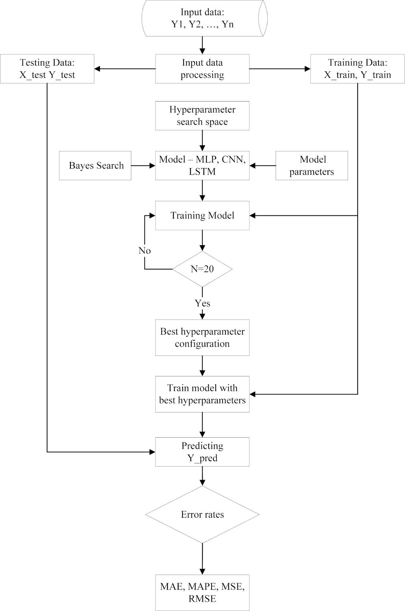
Figure 1. Proposed Framework for Long-Term Electric Load Forecasting Using Bayesian Hyperparameter Optimization
This preprocessing stage is crucial in ensuring the input data are consistent and suitable for training deep learning models. After this step, the hyperparameter search space is defined for the three neural network architectures under investigation—MLP, CNN, and LSTM—in which key hyperparameters such as the number of neurons, filters, batch size, loss function, and number of epochs are specified within particular ranges of values. Subsequently, Bayesian search, implemented through BayesSearchCV, explores the hyperparameter space. During this stage, multiple candidate hyperparameter configurations are generated, and for each configuration, the model is trained and evaluated using time-series cross-validation (TimeSeriesSplit) to ensure objectivity. The process is repeated over 20 trials, and the mean MAPE across folds is recorded at each trial. Once the search process is completed, the best hyperparameter configuration is selected based on the lowest MAPE value. This ensures that the final result is not determined by arbitrary choice but reflects a systematic and rigorous optimization process. With the optimal hyperparameter configuration, the selected model is retrained on the whole training dataset to maximize data utilization. The model is then applied to the test set to generate predicted values (Ŷ_pred), which are directly compared against the actual values of the test set. Finally, a set of error metrics—MAE, MAPE, MSE, and RMSE—is computed to evaluate forecasting performance comprehensively. This workflow offers a structured and scientifically rigorous framework and demonstrates how Bayesian optimization contributes to ensuring fairness in the comparison among MLP, CNN, and LSTM architectures, while simultaneously improving the efficiency of hyperparameter tuning and enhancing the accuracy of long-term electric load forecasting.
- Evaluation Method
This study's evaluation process for long-term load forecasting follows a structured workflow, as illustrated in Figure 1. The procedure begins with raw input data Y1, Y2,…, Yn, which are preprocessed and divided into two subsets: the training set X_train, Y_train, and the testing set X_test, Y_test. After preprocessing, a hyperparameter search space is defined for the three considered deep learning models (MLP, CNN, and LSTM). The Bayesian optimization framework is then employed to explore this search space. At each iteration, the Bayesian search algorithm proposes candidate hyperparameter configurations, which are used to train the forecasting models. The models are evaluated based on validation performance, and the process is repeated for a fixed number of trials. Once the search is completed, the configuration yielding the lowest validation error is selected as the best hyperparameter setting. Using these optimal hyperparameters, the model is retrained from scratch on the whole training dataset. After training, the model generates predictions Y^pred for the test dataset. The accuracy of the forecasts is assessed by comparing predicted values with actual observations. Four standard error metrics are employed: Mean Absolute Error (MAE), Mean Absolute Percentage Error (MAPE), Mean Squared Error (MSE), and Root Mean Square Error (RMSE). These metrics provide a comprehensive evaluation, where MAE and MAPE capture average error magnitude, while MSE and RMSE emphasize large deviations. This multi-metric evaluation ensures that each model's performance is measured regarding average accuracy and robustness to extreme variations.
- RESULT AND DISCUSSION
- Data
The dataset was obtained from the Australian Energy Market Operator (AEMO) for New South Wales (NSW), Australia), covering 01/2015–12/2021 with 2558 daily observations of Peak Load (MW). In this study, we use only Peak Load as the predictor/target (univariate setting); we do not include additional endogenous features (Minimum/Mean/Std) or exogenous variables (weather, holidays). Focusing on Peak Load allows the model to learn directly from the daily demand peak—an operationally critical quantity—while keeping the experimental setup compact and transparent for architectural comparison—definition of long-term. “long-term forecasting” is defined as day-ahead predictions over multi-year horizons. The 2015–2021 period spans pre-, during-, and post-COVID-19, capturing regular seasonality and pandemic-related anomalies. Preprocessing and windowing. The DATE column was standardized to a datetime type and sorted chronologically; the data were checked for missing values (none found). No scaling/normalization was applied (Peak Load remains in MW). We formulate a one-day-ahead task (H = 1 day) with a look-back window K = 365 days: each input sample consists of the sequence [x_(t−364),…,x_t] and the target is y_(t+1). From the original 2558 points, windowing produces 2193 samples (Shape of X = (2193, 365), Shape of y = (2193,).
Time-based split. The series is split chronologically with 80% of the windows for training and 20% for testing (shuffle = False), yielding: Train: X_train (1754, 365), y_train (1754,); Test: X_test (439, 365), y_test (439,). For CNN/LSTM/GRU, inputs are reshaped to (N, 365, 1): X_train→(1754, 365, 1), X_test→(439, 365, 1). For MLP, the flattened (N, 365) representation is used. We did not apply feature scaling or normalization because the peak-load measurements are recorded in consistent, physically meaningful units (MW); transformation methods are beyond the scope of this study and will be considered in future work. Figure 2 illustrates the daily time series of peak load in New South Wales (NSW), Australia, over the period 2015–2021. The plot reveals clear seasonal fluctuations in electricity demand. During summer (December to February), peak load tends to rise due to the intensive use of air conditioning, while in winter (June to August), demand also increases due to heating requirements. By contrast, transitional periods such as spring and autumn exhibit relatively more stable load levels, reflecting reduced influence from extreme climatic conditions.
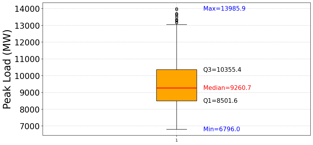
In addition to seasonal cycles, the data also display abrupt fluctuations with abnormal peaks. These spikes are typically associated with extreme weather events such as heatwaves or cold snaps, when the demand for cooling or heating devices surges dramatically. The significant day-to-day variations further highlight the sensitivity of the electricity load to weather conditions, underscoring the strong interdependence between climate and energy consumption. Over the 2015–2021, no clear long-term upward or downward trend in peak load can be observed. Instead, the variability appears to be predominantly driven by seasonal factors and short-term weather conditions rather than a linear growth trajectory. This emphasizes incorporating seasonal and climate-related information into load forecasting models to improve predictive accuracy. Figure 3 presents the boxplot of daily peak load in New South Wales (NSW), Australia, during 2015–2021, highlighting the distributional characteristics of electricity demand. The median peak load is recorded at 9,260.7 MW, representing the typical daily demand level. The interquartile range (IQR), from Q1 = 8,501.6 MW to Q3 = 10,355.4 MW, indicates that 50% of the data are concentrated within this interval, reflecting a relatively stable demand pattern around 9,000–10,000 MW. Beyond the central tendency, the data reveal substantial variability. The minimum observed value is 6,796.0 MW, while the maximum reaches 13,985.9 MW, demonstrating a considerable spread in daily peak demand. Several outliers are also visible above the upper whisker, corresponding to exceptionally high demand days. These extreme cases are often associated with prolonged heatwaves or other adverse weather events, when electricity consumption for cooling sharply increases. Overall, Figure 3 indicates that while most peak load values remain concentrated within a stable range, the electricity system in NSW is subject to frequent fluctuations and occasional extreme surges. This underscores the importance of developing forecasting models that capture average demand patterns and abrupt variations driven by seasonal and climatic factors.
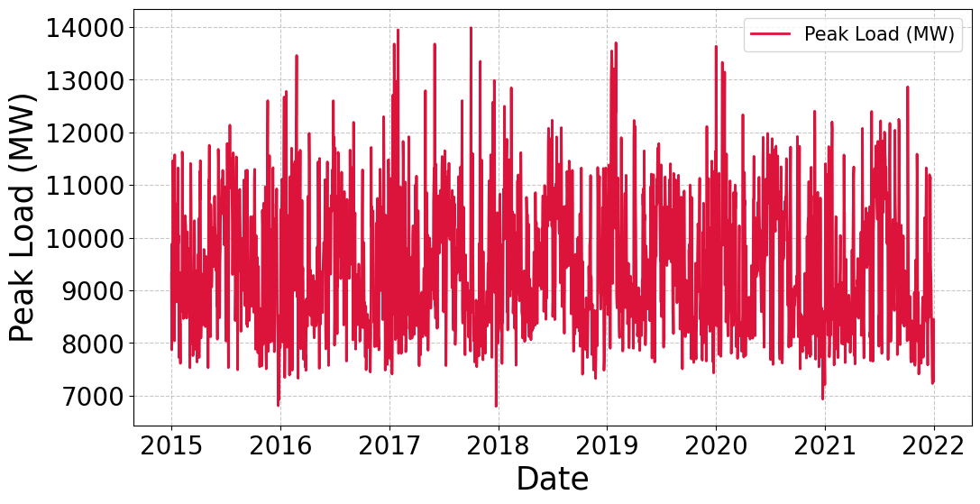
Figure 2. Time Series of Daily Peak Load in NSW (2015–2021)
Figure 3. Boxplot of Daily Peak Load (2015–2021)
- Hyperparameter Grid
Table 1 summarizes the hyperparameter search space designed for the three deep learning models investigated in this study, namely MLP, CNN, and LSTM. Although each model differs in architecture, the search space was constructed consistently and parallel to ensure fairness. For the MLP model, four hidden layers were employed, with the number of neurons in each layer selected from the set {16, 32, 64, 128}. Similarly, in the CNN model, four convolutional layers were configured, and the number of filters was optimized within the same set, thereby maintaining consistency with MLP while reflecting the convolutional nature of the network. The LSTM model followed the same principle, with four LSTM layers, each containing units selected from {16, 32, 64, 128}. The remaining hyperparameters were consistent across the three models to eliminate potential bias. Specifically, the learning rate was fixed at 0.001, which is commonly regarded as a stable starting point for gradient-based optimization in deep neural networks. Two loss functions, Mean Squared Error (MSE) and Mean Absolute Error (MAE), were considered, as they are widely used in regression tasks, particularly in load forecasting; MSE emphasizes significant errors, whereas MAE provides a more robust evaluation against outliers. The batch size was restricted to {16, 32, 64} to balance convergence stability with computational efficiency. Finally, the number of epochs varied between 50 and 250, sufficient to ensure model convergence while avoiding unnecessary training costs. The rationale behind this configuration lies in ensuring both comparability and practicality. By standardizing the search space across MLP, CNN, and LSTM, performance differences can be attributed to the intrinsic learning capability of each architecture rather than discrepancies in hyperparameter tuning. Moreover, the selected ranges are consistent with prior studies on electricity load forecasting, where small- to medium-sized architectures have proven effective in capturing demand dynamics without imposing excessive computational burden. This design thus ensures methodological rigor, computational feasibility, and the generalizability of the results.
Table 1. Hyperparameter Space for MLP, CNN, LSTM
Model | Hyperparameters | Search Space |
MLP
| Neurons per hidden layer (4 layers) | {16, 32, 64, 128} |
Learning rate | {0.001} |
Loss function | {MSE, MAE} |
Batch size | {16, 32, 64} |
Epochs | {50, 100, 150, 200, 250} |
CNN
| Filters per conv layer (4 layers) | {16, 32, 64, 128} |
Learning rate | {0.001} |
Loss function | {MSE, MAE} |
Batch size | {16, 32, 64} |
Epochs | {50, 100, 150, 200, 250} |
LSTM
| Units per LSTM layer (4 layers) | {16, 32, 64, 128} |
Learning rate | {0.001} |
Loss function | {MSE, MAE} |
Batch size | {16, 32, 64} |
Epochs | {50, 100, 150, 200, 250} |
- Evaluation Outcomes
Figure 4 presents the forecasting performance of the optimized MLP model on the test dataset, where the actual load values are compared against the predicted outputs. After Bayesian hyperparameter tuning, the results demonstrate that the MLP model can capture the overall dynamics of electricity demand, including general trends and seasonal fluctuations. The predicted series aligns relatively well with the actual values, particularly in periods of stable demand, which indicates that the MLP can effectively learn the dominant patterns in the data. However, the figure also highlights notable discrepancies at extreme load conditions. Specifically, the model underestimates sharp peaks during high-demand periods and slightly overestimates troughs in low-demand intervals. These deviations suggest that while the MLP architecture is efficient in modeling nonlinear relationships, its feedforward structure may be less effective in representing temporal dependencies and abrupt changes inherent in load demand. The optimized MLP provides a solid baseline performance for long-term load forecasting.
Figure 5 presents the forecasting performance of the optimized LSTM model on the test dataset, where the actual load demand is compared against the predicted values. The results indicate that the LSTM model can effectively capture the underlying temporal dynamics of electricity consumption, including recurring trends and seasonal fluctuations. Owing to its recurrent architecture, the LSTM demonstrates stronger capability in modeling sequential dependencies than feedforward structures, enabling the predicted series to align closely with the actual demand during periods of gradual variation. However, the figure also reveals discrepancies at extreme conditions. The model underestimates sharp peaks during high-demand intervals and fails to fully reproduce the magnitude of sudden load drops. These deviations suggest that while the LSTM excels in learning long-term temporal correlations and nonlinear relationships, it remains less responsive to abrupt fluctuations and outlier events. Overall, the optimized LSTM provides reliable forecasting accuracy and a robust approach for long-term load prediction. However, further refinement may be necessary to enhance its ability to capture extreme demand variations.
Figure 6 presents the forecasting performance of the optimized CNN model on the test dataset, where the actual load values are compared against the predicted outputs. After Bayesian hyperparameter tuning, the results show that the CNN model can effectively capture the overall dynamics of electricity demand, including both long-term trends and short-term fluctuations. The predicted series strongly aligns with the actual values, particularly in segments with moderate demand, indicating that the CNN architecture can successfully extract local temporal features through its convolutional layers. However, discrepancies remain visible at extreme load conditions. In particular, the model occasionally underestimates sharp demand peaks and slightly overestimates certain low-demand intervals. These deviations suggest that while CNN excels in capturing localized patterns and improving predictive accuracy compared to simpler feedforward models, it may still face challenges in fully representing highly volatile or abrupt changes in load behaviour. Overall, the optimized CNN delivers robust forecasting accuracy and demonstrates the effectiveness of Bayesian hyperparameter search in enhancing its performance for long-term electric load forecasting.
Table 2 shows a consistent performance ranking across the three architectures, with CNN achieving the best results on all metrics, MLP second, and LSTM the worst. Specifically, CNN attains MAE = 699, lower than MLP (746, a difference of ≈ 6.7%) and LSTM (909, ≈ 30%). On metrics sensitive to large deviations, CNN’s MSE/RMSE (791,838/890) also outperforms MLP (940,334/970) and especially LSTM (1,309,799/1,144), indicating better control over extreme errors. In terms of relative error, CNN’s MAPE is 7.53%, better than MLP (8.02%, +0.49 percentage points ~ +6.5% relative) and LSTM (9.74%, +2.21 percentage points ~ +29.3% relative). The agreement in ranking across all metrics (CNN < MLP < LSTM) supports the conclusion that, under the univariate day-ahead setup with a 365-day window, CNN delivers higher and more stable accuracy; MLP is close but still noticeably worse on squared-error metrics, whereas LSTM yields the most significant errors—suggesting that the limited tuning budget and/or current hyperparameter choices have not effectively leveraged the long-term dependency modeling of sequential architectures. The gaps between CNN and LSTM across all metrics are markedly larger than the inter–fold variation, indicating practical significance for long-term deployment. CNN also consistently outperforms MLP by smaller yet stable margins across all metrics. Figure 7 compares runtime performance among the MLP, CNN, and LSTM models after Bayesian hyperparameter optimization in long-term electric load forecasting. The results show that the MLP model required 726 seconds, the CNN model took 900 seconds, and the LSTM model consumed 8,900 seconds. The chart highlights a significant difference in runtime across the three models, with MLP and CNN showing relatively low execution times. At the same time, LSTM required considerably more computation time. This distribution reflects the computational cost of each model during training and forecasting.
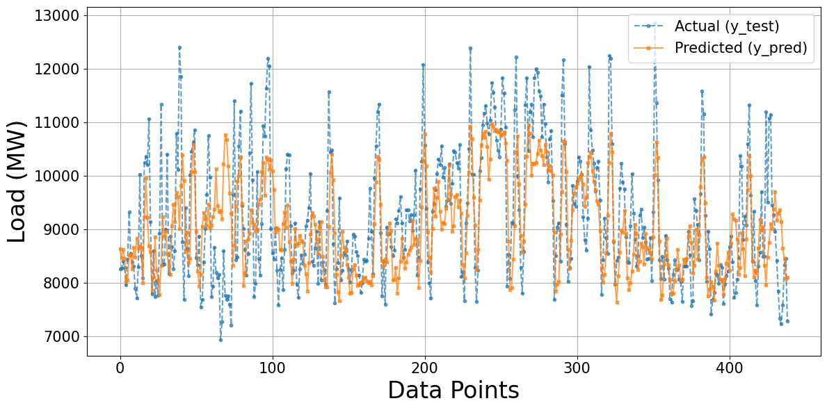
Figure 4. Actual vs predicted load using the MLP model optimized with Bayesian Search
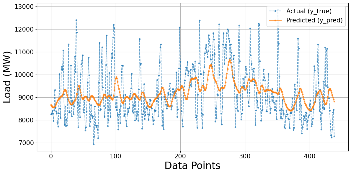
Figure 5. Actual vs predicted load using the LSTM model optimized with Bayesian Search
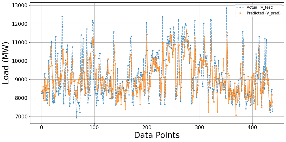
Figure 6. Actual vs predicted load using the CNN model optimized with Bayesian Search
Table 2. Model performance on NSW data (2015–2021) for MLP, LSTM, and CNN
Metric | MLP | CNN | LSTM |
MAE | 746.00 | 699 | 909 |
MSE | 940,334 | 791,838 | 1,309,799 |
RMSE | 970 | 890 | 1,144 |
MAPE (%) | 8.02 | 7.53 | 9.74 |
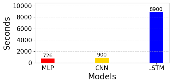
Figure 7. Runtime Across Models
- Discussion
The experimental results in Table 2 reveal apparent differences among the MLP, CNN, and LSTM models in the long-term electric load forecasting task. Although LSTM has traditionally been considered a common choice for time series tasks due to its ability to model long-term dependencies, the findings of this study indicate that its performance in long-term load forecasting is not as effective as expected. This limitation can be attributed to the characteristics of load data, which contain strong local fluctuations, seasonal variations, and abrupt changes. In such cases, the recurrent structure of LSTM is prone to vanishing gradient issues, thereby reducing its ability to fully capture complex variations across extended horizons. In contrast, CNN appears more suitable due to its ability to extract local and hierarchical features, enabling the effective modelling of short-term and long-term patterns. The lower error values and reasonable training time obtained by CNN reinforce the view that convolution-based architectures are efficient in image processing and can adapt well to complex time series tasks such as electric load forecasting. Furthermore, MLP, despite being structurally simpler, still demonstrated stable results, making it a useful baseline model for comparative studies.
Another important aspect is the significant difference in computational cost. LSTM required considerably longer training time than CNN and MLP, which reduces its practicality for large-scale deployment or applications where rapid response is essential. As such, LSTM did not demonstrate predictive accuracy or computational efficiency advantages in long-term load forecasting. These findings suggest several directions for future improvement. One potential solution is the development of hybrid CNN–LSTM models, where CNN is responsible for extracting local features and LSTM for capturing long-term dependencies. Additionally, the recent advancements of Transformer-based models, such as the Temporal Fusion Transformer (TFT) and Informer, offer promising alternatives due to their ability to model long-term dependencies without suffering from vanishing gradient problems. Integrating such architectures with advanced hyperparameter optimization strategies could further enhance the accuracy and efficiency of long-term electric load forecasting in future research. Although no formal tests are conducted, the observed differences exceed inter-fold variability and persist across all metrics, suggesting a tangible benefit of choosing CNN (or MLP) for operational settings. This study does not include formal statistical significance testing (Diebold–Mariano tests) or bootstrap confidence intervals. We leave these analyses for future work. We do not include seasonal/persistence baselines, as the study is scoped to the comparative effect of Bayesian optimization across learned models. Future work will complement these results with a broader baseline benchmark.
- CONCLUSIONS
This study evaluated MLP, CNN, and LSTM under a unified Bayesian hyperparameter optimization protocol for long-term electric load forecasting. The CNN architecture consistently achieved the highest accuracy across standard error metrics (MAE, MSE, RMSE, MAPE). At the same time, MLP delivered comparable performance at lower architectural complexity, and LSTM exhibited the most significant errors and computational cost. These findings underscore the value of Bayesian optimization for establishing a fair comparison baseline and improving model effectiveness in long-horizon settings. A practical implication is that CNN is a strong default choice for long-term planning scenarios, with MLP as a viable alternative when resources are constrained. The present work is limited by a univariate setup and a modest search budget; future research will examine multivariate inputs (weather and calendar effects), larger or adaptive search budgets, and advanced or hybrid architectures (CNN–LSTM and Transformers) to enhance forecasting accuracy and generalizability further.
REFERENCES
- G. F. Fan, G. F. Fan, R. T. Zhang, C. C. Cao, Y. H. Yeh, and W. C. Hong, “Applications of empirical wavelet decomposition, statistical feature extraction, and antlion algorithm with support vector regression for resident electricity consumption forecasting,” Nonlinear Dyn., vol. 111, no. 21, pp. 20139–20163, 2023, https://doi.org/10.1007/s11071-023-08922-9.
- W. Lizhen, Z. Yifan, W. Gang, and H. Xiaohong, “A novel short-term load forecasting method based on mini-batch stochastic gradient descent regression model,” Electr. Power Syst. Res., vol. 211, no. November 2021, p. 108226, 2022, https://doi.org/10.1016/j.epsr.2022.108226.
- L. Han, P. Pinson, and J. Kazempour, “Trading data for wind power forecasting: A regression market with lasso regularization,” Electr. Power Syst. Res., vol. 212, no. October 2021, p. 108442, 2022, https://doi.org/10.1016/j.epsr.2022.108442.
- A. Petrusic and A. Janjic, “Fuzzy Multiple Linear Regression for the Short Term Load Forecast,” 2020 55th Int. Sci. Conf. Information, Commun. Energy Syst. Technol. ICEST 2020 - Proc., pp. 102–105, 2020, https://doi.org/10.1109/ICEST49890.2020.9232776.
- P. Ran, K. Dong, X. Liu, and J. Wang, “Short-term load forecasting based on CEEMDAN and Transformer,” Electr. Power Syst. Res., vol. 214, no. PA, p. 108885, 2023, https://doi.org/10.1016/j.epsr.2022.108885.
- A. Gupta and A. Kumar, “Mid-Term Daily Load Forecasting using ARIMA, Wavelet-ARIMA and Machine Learning,” Proc. - 2020 IEEE Int. Conf. Environ. Electr. Eng. 2020 IEEE Ind. Commer. Power Syst. Eur. EEEIC / I CPS Eur. 2020, pp. 0–4, 2020, https://doi.org/10.1109/EEEIC/ICPSEurope49358.2020.9160563.
- Y. Miao and Z. Chen, “Short-term Load Forecasting Based on Echo State Network and LightGBM,” 2023 IEEE Int. Conf. Predict. Control Electr. Drives Power Electron., no. 52177087, pp. 1–6, 2023, https://doi.org/10.1109/PRECEDE57319.2023.10174609.
- J. A. C. Dias et al., “Enhanced Carbon Flux Forecasting via STL Decomposition and Hybrid ARIMA-ES-LSTM Model in Amazon Forest,” IEEE Access, vol. 13, no. February, pp. 84713–84726, 2025, https://doi.org/10.1109/ACCESS.2025.3561166.
- S. Chen, R. Lin, and W. Zeng, “Short-Term Load Forecasting Method Based on ARIMA and LSTM,” Int. Conf. Commun. Technol. Proceedings, ICCT, vol. 2022-Novem, pp. 1913–1917, 2022, https://doi.org/10.1109/ICCT56141.2022.10073051.
- U. Samal and A. Kumar, “Enhancing Software Reliability Forecasting Through a Hybrid ARIMA-ANN Model,” Arab. J. Sci. Eng., 2023, https://doi.org/10.1007/s13369-023-08486-1.
- A. P. Wibawa, A. B. P. Utama, H. Elmunsyah, U. Pujianto, F. A. Dwiyanto, and L. Hernandez, “Time-series analysis with smoothed Convolutional Neural Network,” J. Big Data, vol. 9, no. 1, 2022, https://doi.org/10.1186/s40537-022-00599-y.
- U. I. Lezama Lope, A. Benavides-Vázquez, G. Santamaría-Bonfil, and R. Z. Ríos-Mercado, “Fast and Efficient Very Short-Term Load Forecasting Using Analogue and Moving Average Tools,” IEEE Lat. Am. Trans., vol. 21, no. 9, pp. 1015–1021, 2023, https://doi.org/10.1109/tla.2023.10251808.
- R. Bitit, A. Derhab, M. Guerroumi, and F. A. Khan, “DDoS attack forecasting based on online multiple change points detection and time series analysis,” Multimed. Tools Appl., vol. 83, no. 18, pp. 53655–53685, 2024, https://doi.org/10.1007/s11042-023-17637-3.
- N. T. Dieudonné, T. K. F. Armel, A. K. C. Vidal, and T. René, “Prediction of electrical energy consumption in Cameroon through econometric models,” Electr. Power Syst. Res., vol. 210, no. May, 2022, https://doi.org/10.1016/j.epsr.2022.108102.
- S. A. Mousavi and M. Gholami, “Optimized load vector regression for load prediction and improvement using trombe walls in household electrical energy consumption,” Energy Effic., vol. 17, no. 7, 2024, https://doi.org/10.1007/s12053-024-10252-7.
- Z. Zhang, Y. Dong, and W. C. Hong, “Long Short-Term Memory-Based Twin Support Vector Regression for Probabilistic Load Forecasting,” IEEE Trans. Neural Networks Learn. Syst., vol. 36, no. 1, pp. 1764–1778, 2023, https://doi.org/10.1109/TNNLS.2023.3335355.
- H. Liu, Y. Tang, Y. Pu, F. Mei, and D. Sidorov, “Short-term Load Forecasting of Multi-Energy in Integrated Energy System Based on Multivariate Phase Space Reconstruction and Support Vector Regression Mode,” Electr. Power Syst. Res., vol. 210, no. April, p. 108066, 2022, https://doi.org/10.1016/j.epsr.2022.108066.
- Y. Lu and G. Wang, “A load forecasting model based on support vector regression with whale optimization algorithm,” Multimed. Tools Appl., vol. 82, no. 7, pp. 9939–9959, 2023, https://doi.org/10.1007/s11042-022-13462-2.
- A. Lindholm, N. Wahlström, F. Lindsten, and T. B. Schön, “Machine Learning,” Mach. Learn., 2022, https://doi.org/10.1017/9781108919371.
- M. Goyal and M. Pandey, “A Systematic Analysis for Energy Performance Predictions in Residential Buildings Using Ensemble Learning,” Arab. J. Sci. Eng., vol. 46, no. 4, pp. 3155-3168, 2020, https://doi.org/10.1007/s13369-020-05069-2.
- R. Banik and A. Biswas, “Enhanced renewable power and load forecasting using RF-XGBoost stacked ensemble,” Electr. Eng., vol. 106, no. 4, pp. 4947–4967, 2024, https://doi.org/10.1007/s00202-024-02273-3.
- D. Barochiner, R. Lado, L. Carletti, and F. Pintar, “A machine learning approach to address 1-week-ahead peak demand forecasting using the XGBoost algorithm,” 2022 IEEE Bienn. Congr. Argentina, ARGENCON 2022, 2022, https://doi.org/10.1109/ARGENCON55245.2022.9939986.
- L. Semmelmann, S. Henni, and C. Weinhardt, “Load forecasting for energy communities: a novel LSTM-XGBoost hybrid model based on smart meter data,” Energy Informatics, vol. 5, no. 1, pp. 1–21, 2022, https://doi.org/10.1186/s42162-022-00212-9.
- S. Lei and F. Wang, “A Two-stage Short-term Load Forecasting Method Based on Comprehensive Similarity Day Selection and CEEMDAN-XGBoost Error Correction,” 2023 Int. Conf. Futur. Energy Solut., pp. 1–6, https://doi.org/10.1109/FES57669.2023.10183307.
- M. Abdurohman and A. G. Putrada, “Forecasting Model for Lighting Electricity Load with a Limited Dataset using XGBoost,” Kinet. Game Technol. Inf. Syst. Comput. Network, Comput. Electron. Control, vol. 8, no. 2, pp. 571–580, 2023, https://doi.org/10.22219/kinetik.v8i2.1687.
- S. Wang and J. Ma, “A Novel Ensemble Model for Load Forecasting: Integrating Random Forest, XGBoost, and Seasonal Naive Methods,” Proc. - 2023 2nd Asian Conf. Front. Power Energy, ACFPE 2023, pp. 114–118, 2023, https://doi.org/10.1109/ACFPE59335.2023.10455494.
- Q. Yang, Y. Lin, S. Kuang, and D. Wang, “A novel short-term load forecasting approach for data-poor areas based on K-MIFS-XGBoost and transfer-learning,” Electr. Power Syst. Res., vol. 229, no. January, p. 110151, 2024, https://doi.org/10.1016/j.epsr.2024.110151.
- J. Zhang, Z. Zhu, and Y. Yang, “Electricity Load Forecasting Based on CNN-LSTM,” 2023 IEEE Int. Conf. Electr. Autom. Comput. Eng. ICEACE 2023, pp. 1385–1390, 2023, https://doi.org/10.1109/ICEACE60673.2023.10442217.
- Z. Liao, H. Pan, X. Fan, Y. Zhang, and L. Kuang, “Multiple Wavelet Convolutional Neural Network for Short-Term Load Forecasting,” IEEE Internet Things J., vol. 8, no. 12, pp. 9730–9739, 2021, https://doi.org/10.1109/JIOT.2020.3026733.
- T. Bashir, H. Wang, M. Tahir, and Y. Zhang, “Wind and solar power forecasting based on hybrid CNN-ABiLSTM, CNN-transformer-MLP models,” Renew. Energy, vol. 239, no. August 2024, p. 122055, 2025, https://doi.org/10.1016/j.renene.2024.122055.
- A. Agga, A. Abbou, M. Labbadi, and Y. El Houm, “Short-Term Load Forecasting: Based on Hybrid CNN-LSTM Neural Network,” 2021 6th Int. Conf. Power Renew. Energy, ICPRE 2021, pp. 886–891, 2021, https://doi.org/10.1109/ICPRE52634.2021.9635488.
- O. Rubasinghe et al., “A Novel Sequence to Sequence Data Modelling Based CNN-LSTM Algorithm for Three Years Ahead Monthly Peak Load Forecasting,” IEEE Trans. Power Syst., vol. 39, no. 2, pp. 1932–1947, 2024, https://doi.org/10.1109/TPWRS.2023.3271325.
- Z. Tian, W. Liu, W. Jiang, and C. Wu, “CNNs-Transformer based day-ahead probabilistic load forecasting for weekends with limited data availability,” vol. 293, no. September 2023, p. 130666, 2024, https://doi.org/10.1016/j.energy.2024.130666.
- A. Irankhah, S. R. Saatlou, M. H. Yaghmaee, S. Ershadi-Nasab, and M. Alishahi, “A parallel CNN-BiGRU network for short-term load forecasting in demand-side management,” 2022 12th Int. Conf. Comput. Knowl. Eng. ICCKE 2022, no. Iccke, pp. 511–516, 2022, https://doi.org/10.1109/ICCKE57176.2022.9960036.
- M. Alhussein, K. Aurangzeb, and S. I. Haider, “Hybrid CNN-LSTM Model for Short-Term Individual Household Load Forecasting,” IEEE Access, vol. 8, pp. 180544–180557, 2020, https://doi.org/10.1109/ACCESS.2020.3028281.
- M. Aouad, H. Hajj, K. Shaban, R. A. Jabr, and W. El-Hajj, “A CNN-Sequence-to-Sequence network with attention for residential short-term load forecasting,” Electr. Power Syst. Res., vol. 211, no. June, p. 108152, 2022, https://doi.org/10.1016/j.epsr.2022.108152.
- S. H. Rafi, N. Al-Masood, S. R. Deeba, and E. Hossain, “A short-term load forecasting method using integrated CNN and LSTM network,” IEEE Access, vol. 9, pp. 32436–32448, 2021, https://doi.org/10.1109/ACCESS.2021.3060654.
- C. Fan, Y. Li, L. Yi, L. Xiao, X. Qu, and Z. Ai, “Multi-objective LSTM ensemble model for household short-term load forecasting,” Memetic Comput., vol. 14, no. 1, pp. 115–132, 2022, https://doi.org/10.1007/s12293-022-00355-y.
- Y. Yang, E. U. Haq, and Y. Jia, “A Novel Deep Learning Approach for Short and Medium-Term Electrical Load Forecasting Based on Pooling LSTM-CNN Model,” 2020 IEEE/IAS Ind. Commer. Power Syst. Asia, I CPS Asia 2020, pp. 26–34, 2020, https://doi.org/10.1109/ICPSAsia48933.2020.9208557.
- Q. Liu, J. Cao, J. Zhang, Y. Zhong, T. Ba, and Y. Zhang, “Short-Term Power Load Forecasting in FGSM-Bi-LSTM Networks Based on Empirical Wavelet Transform,” IEEE Access, vol. 11, no. September, pp. 105057–105068, 2023, https://doi.org/10.1109/ACCESS.2023.3316516.
- J. Wen, Y. Peng, W. Zhang, X. Huang, and Z. Wang, “Short-term power load forecasting based on TCN-LSTM model,” Proc. 2024 IEEE 6th Int. Conf. Civ. Aviat. Saf. Inf. Technol. ICCASIT 2024, pp. 734–738, 2024, https://doi.org/10.1109/ICCASIT62299.2024.10827868.
- M. Munem, T. M. Rubaith Bashar, M. H. Roni, M. Shahriar, T. B. Shawkat, and H. Rahaman, “Electric power load forecasting based on multivariate LSTM neural network using bayesian optimization,” 2020 IEEE Electr. Power Energy Conf. EPEC 2020, vol. 3, pp. 5–10, 2020, https://doi.org/10.1109/EPEC48502.2020.9320123.
- X. Yang and Z. Chen, “A Hybrid Short-Term Load Forecasting Model Based on CatBoost and LSTM,” 2021 IEEE 6th Int. Conf. Intell. Comput. Signal Process. ICSP 2021, no. Icsp, pp. 328–332, 2021, https://doi.org/10.1109/ICSP51882.2021.9408768.
- A. Faustine, N. J. Nunes, and L. Pereira, “Efficiency through Simplicity: MLP-based Approach for Net-Load Forecasting with Uncertainty Estimates in Low-Voltage Distribution Networks,” IEEE Trans. Power Syst., vol. 40, no. 1, pp. 46–56, 2024, https://doi.org/10.1109/TPWRS.2024.3400123.
- J. H. Kim, B. S. Lee, and C. H. Kim, “A Study on the development of long-term hybrid electrical load forecasting model based on MLP and statistics using massive actual data considering field applications,” Electr. Power Syst. Res., vol. 221, no. April, p. 109415, 2023, https://doi.org/10.1016/j.epsr.2023.109415.
- S. C. Pall, S. H. Cheragee, M. R. Mahamud, H. M. Mishu, and H. Biswas, “Performance Analysis of Machine Learning and ANN for Load Forecasting in Bangladesh,” 2023 Int. Conf. Next-Generation Comput. IoT Mach. Learn. NCIM 2023, no. June, pp. 1–5, 2023, https://doi.org/10.1109/NCIM59001.2023.10212451.
- I. C. Figueiró, A. R. Abaide, N. K. Neto, L. N. F. Silva, and L. L. C. Santos, “Bottom-Up Short-Term Load Forecasting Considering Macro-Region and Weighting by Meteorological Region,” Energies, vol. 16, no. 19, pp. 1191–1198, 2023, https://doi.org/10.3390/en16196857.
- H. Tong and J. Liu, “MFformer: An improved transformer-based multi-frequency feature aggregation model for electricity load forecasting,” Electr. Power Syst. Res., vol. 243, no. September 2024, p. 111492, 2025, https://doi.org/10.1016/j.epsr.2025.111492.
- J. Yang, “Accurate cooling load estimation using multi-layer perceptron machine learning models,” Signal, Image Video Process., vol. 18, no. 11, pp. 7711–7727, 2024, https://doi.org/10.1007/s11760-024-03422-8.
- I. Diahovchenko, A. Chuprun, and Z. Čonka, “Assessment and mitigation of the influence of rising charging demand of electric vehicles on the aging of distribution transformers,” Electr. Power Syst. Res., vol. 221, no. May, 2023, https://doi.org/10.1016/j.epsr.2023.109455.
- J. Gao, Y. Chen, W. Hu, and D. Zhang, “An adaptive deep-learning load forecasting framework by integrating transformer and domain knowledge,” Adv. Appl. Energy, vol. 10, no. February, p. 100142, 2023, https://doi.org/10.1016/j.adapen.2023.100142.
- H. Liao and K. K. Radhakrishnan, “Short-Term Load Forecasting with Temporal Fusion Transformers for Power Distribution Networks,” Proc. - 2022 IEEE Sustain. Power Energy Conf. iSPEC 2022, pp. 1–5, 2022, https://doi.org/10.1109/iSPEC54162.2022.10033079.
- C. Feng, L. Shao, J. Wang, Y. Zhang, and F. Wen, “Short-term Load Forecasting of Distribution Transformer Supply Zones Based on Federated Model-Agnostic Meta Learning,” IEEE Trans. Power Syst., vol. 40, no. 1, pp. 31–45, 2024, https://doi.org/10.1109/TPWRS.2024.3393017.
- C. Xu and G. Chen, “Interpretable transformer-based model for probabilistic short-term forecasting of residential net load,” Int. J. Electr. Power Energy Syst., vol.. 155, no. PB, p. 109515, 2024, https://doi.org/10.1016/j.ijepes.2023.109515.
- L. Li, X. Su, X. Bi, Y. Lu, and X. Sun, “A novel Transformer-based network forecasting method for building cooling loads,” Energy Build., vol. 296, no. July, p. 113409, 2023, https://doi.org/10.1016/j.enbuild.2023.113409.
- H. Zhao, Y. Wu, L. Ma, and S. Pan, “Spatial and Temporal Attention-Enabled Transformer Network for Multivariate Short-Term Residential Load Forecasting,” IEEE Trans. Instrum. Meas., vol. 72, pp. 1–11, 2023, https://doi.org/10.1109/TIM.2023.3305655.
- G. Tziolis et al., “Short-term electric net load forecasting for solar-integrated distribution systems based on Bayesian neural networks and statistical post-processing,” Energy, vol. 271, no. February, p. 127018, 2023, https://doi.org/10.1016/j.energy.2023.127018.
- C. Wang, Y. Wang, Z. Ding, and K. Zhang, “Probabilistic Multi-energy Load Forecasting for Integrated Energy System Based on Bayesian Transformer Network,” IEEE Trans. Smart Grid, vol. 15, no. 2, pp. 1495–1508, 2023, https://doi.org/10.1109/TSG.2023.3296647.
- V. Urošević and A. M. Savić, “Temporal clustering for accurate short-term load forecasting using Bayesian multiple linear regression,” Appl. Intell., vol. 55, no. 1, 2025, https://doi.org/10.1007/s10489-024-05887-z.
- D. Kiruthiga and V. Manikandan, “Intraday time series load forecasting using Bayesian deep learning method—a new approach,” Electr. Eng., vol. 104, no. 3, pp. 1697–1709, 2022, https://doi.org/10.1007/s00202-021-01411-5.
- M. Vijay and M. Saravanan, “Solar Irradiance Forecasting using Bayesian Optimization based Machine Learning Algorithm to Determine the Optimal Size of a Residential PV System,” Int. Conf. Sustain. Comput. Data Commun. Syst. ICSCDS 2022 - Proc., pp. 744–749, 2022, https://doi.org/10.1109/ICSCDS53736.2022.9761011.
- M. A. Iqbal, J. M. Gil, and S. K. Kim, “Attention-Driven Hybrid Ensemble Approach with Bayesian Optimization for Accurate Energy Forecasting in Jeju Island’s Renewable Energy System,” IEEE Access, vol. 13, no. January, pp. 7986–8010, 2025, https://doi.org/10.1109/ACCESS.2025.3526943.
- X. Li, H. Guo, L. Xu, and Z. Xing, “Bayesian-Based Hyperparameter Optimization of 1D-CNN for Structural Anomaly Detection,” Sensors, vol. 23, no. 11, 2023, https://doi.org/10.3390/s23115058.
AUTHOR BIOGRAPHY

| Nguyen Anh Tuan     received a B.Sc. degree from the Industrial University of Ho Chi Minh City, Vietnam 2012, and an M.Sc. degree from the HCMC University of Technology and Education, Vietnam, in 2015. He is a Lecturer with the Faculty of Electrical Engineering Technology at the Industrial University of Ho Chi Minh City, Vietnam. His main research interests include power quality and load forecasting. received a B.Sc. degree from the Industrial University of Ho Chi Minh City, Vietnam 2012, and an M.Sc. degree from the HCMC University of Technology and Education, Vietnam, in 2015. He is a Lecturer with the Faculty of Electrical Engineering Technology at the Industrial University of Ho Chi Minh City, Vietnam. His main research interests include power quality and load forecasting. Email: nguyenanhtuan@iuh.edu.vn |
|
|

| Trung Dung Nguyen was born in 1976 in Vietnam. He received a Master’s degree in Electrical Engineering from Ho Chi Minh City University of Technology and Education, Vietnam, in 2017. He lectures at the Faculty of Electrical Engineering Technology, Industrial University of Ho Chi Minh City, Ho Chi Minh City, Vietnam. His research focuses on applications of metaheuristic algorithms in power system optimization, optimal control, and model predictive control. Email: nguyentrungdung@iuh.edu.vn |
Tuan Anh Nguyen (Bayesian-Optimized MLP-LSTM-CNN for Multi-Year Day-Ahead Electric Load Forecasting)