Buletin Ilmiah Sarjana Teknik Elektro ISSN: 2685-9572
Vol. 7, No. 3, September 2025, pp. 481-495
Analysis of Swarm Size and Iteration Count in Particle Swarm Optimization for Convolutional Neural Network Hyperparameter Optimization in Short-Term Load Forecasting
Tuan Anh Nguyen, Trung Dung Nguyen
FEET, Industrial University of Ho Chi Minh City, Ho Chi Minh City, Viet Nam
ARTICLE INFORMATION |
| ABSTRACT |
Article History: Received 12 June 2025 Revised 31 July 2025 Accepted 08 September 2025 |
| 
Short-term load forecasting (STLF) is critical in modern power system planning and operation. However, the effectiveness of deep learning models such as Convolutional Neural Networks (CNNs) depends on selecting hyperparameters, which are traditionally tuned through time-consuming trial-and-error processes. The research contribution of this study is to systematically analyze how two key parameters—swarm size and iteration count—in Particle Swarm Optimization (PSO) affect the performance of CNN hyperparameter tuning for STLF. A CNN architecture with fixed convolutional depth is optimized using PSO over selected hyperparameters, including the number of filters, batch size, and training epochs. The experiments use two regional Australian electricity load datasets: New South Wales (NSW) and Queensland (QLD). A three-fold cross-validation strategy is employed, and the Mean Absolute Percentage Error (MAPE) is used as the primary evaluation metric. The results show that optimal PSO configurations vary significantly between datasets, with smaller swarm sizes and moderate iteration counts yielding favorable trade-offs between forecasting accuracy and computational cost. However, the reliance on MAPE, sensitivity to near-zero values, and fixed CNN architecture impose limitations. This study provides practical guidance for selecting PSO settings in deep learning-based STLF and demonstrates that tuning PSO configurations can significantly enhance model performance while reducing computational overhead. Future work may explore adaptive or hybrid optimization methods and extend to more diverse forecasting scenarios. |
Keywords: Particle Swarm Optimization; Convolutional Neural Networks Load Forecasting; Hyperparameter Optimization; Time Series Forecasting |
Corresponding Author: Trung Dung Nguyen,
FEET, Industrial University of Ho Chi Minh City, Ho Chi Minh City, Viet Nam.
Email: nguyentrungdung@iuh.edu.vn |
This work is licensed under a Creative Commons Attribution-Share Alike 4.0 
|
Document Citation: T. A. Nguyen and T. D. Nguyen, “Analysis of Swarm Size and Iteration Count in Particle Swarm Optimization for Convolutional Neural Network Hyperparameter Optimization in Short-Term Load Forecasting,” Buletin Ilmiah Sarjana Teknik Elektro, vol. 7, no. 3, pp. 481-495, 2025, DOI: 10.12928/biste.v7i3.13953. |
INTRODUCTION
Short-term load forecasting (STLF) plays a critical role in ensuring modern power systems' operational reliability and economic efficiency. Accurate load forecasts support better generation scheduling, system balancing, and demand response planning. Even minor forecasting improvements can result in measurable operational cost savings and grid stability gains. Traditional forecasting methods, including statistical approaches [1][2], and shallow machine learning models such as ARIMA, SARIMA [3]–[8], and regression-based techniques [9][10], have been extensively studied. However, these models often fall short when faced with nonlinearities, seasonality, and the stochastic nature of electricity consumption patterns influenced by weather, calendar events, and user behavior.
Deep learning models have emerged as effective alternatives in recent years by automatically learning representations from raw time series data. Multilayer Perceptron (MLP) [11]–[14] was one of the earliest deep models applied to load forecasting, offering basic nonlinear mapping capabilities. However, its lack of memory severely limits performance on temporal data. Long Short-Term Memory (LSTM) networks [15]–[18], designed to retain long-range dependencies, addressed this issue but introduced challenges related to high computational cost and longer training times. Convolutional Neural Networks (CNNs) [19]–[23], initially designed for spatial data, have been successfully adapted for time series by treating historical load sequences as one-dimensional signals. CNNs are known for extracting localized temporal features and offering superior training efficiency compared to recurrent models, making them suitable for real-time forecasting applications. More recently, Transformer-based models [24]–[27], including Informer and Autoformer, have advanced the state of the art in STLF by leveraging self-attention mechanisms for global context modeling and faster parallel training. Additionally, hybrid models such as CNN–LSTM combinations [33]–[36], GRU-based architectures [28]–[32], and attention-enhanced frameworks have been proposed further to improve accuracy and robustness under diverse data conditions.
Despite these advancements, hyperparameter tuning remains one of the most challenging aspects of applying deep learning in STLF. CNN performance can vary significantly depending on design and training hyperparameters, including the number of filters, learning rate, batch size, and epochs. Conventional optimization techniques such as grid search [37]–[39] and random search [40][41] are often computationally inefficient and may miss near-optimal solutions. As a result, recent studies have turned to metaheuristic optimization methods such as Particle Swarm Optimization (PSO) [42][43], which balance exploration and exploitation to tune hyperparameters in complex search spaces effectively. PSO is a population-based stochastic optimization algorithm inspired by the collective behavior of bird flocks. It uses personal and group knowledge to adjust candidate solutions (particles) over successive iterations. In load forecasting, PSO has been successfully applied to optimize SVR [44][45], neural network architectures, and hybrid model components. However, its effectiveness depends heavily on selecting internal control parameters—most notably the swarm size (number of particles) and the number of iterations. A larger swarm allows broader search space coverage but increases per-iteration computational cost. Conversely, small swarm sizes reduce cost but risk suboptimal convergence. Similarly, more iterations may enhance accuracy up to a point, but excessive training can lead to diminishing returns or overfitting.
While PSO has been widely used as an optimization tool, there is limited analysis on how different configurations of swarm size and iteration count influence its performance in deep learning hyperparameter tuning, particularly in STLF tasks. This research addresses that gap by systematically evaluating how varying PSO parameters affect the tuning of CNN hyperparameters for STLF on real-world electricity demand datasets from New South Wales (NSW) and Queensland (QLD), Australia. The research contribution is as follows: (1) A comprehensive analysis of how PSO control parameters influence CNN optimization quality and runtime efficiency in load forecasting tasks; (2) An empirical evaluation of performance trade-offs across multiple PSO configurations using 3-fold cross-validation and Mean Absolute Percentage Error (MAPE) as the primary metric; (3) Practical guidelines for selecting PSO settings tailored to data complexity and available computational resources. This study contributes to understanding metaheuristic design in deep learning applications and offers actionable insights for researchers and practitioners seeking to enhance forecasting models through efficient hyperparameter optimization.
THEORETICAL BACKGROUND
Convolutional Neural Network
Convolutional Neural Networks (CNNs) are deep learning models with outstanding performance in processing grid-structured data, particularly in image analysis and one-dimensional time series. Initially widely used in computer vision tasks such as face recognition, object classification, and localization, CNN architectures have also been successfully extended to short-term load forecasting (STLF) applications. A typical CNN model consists of four core components: convolutional layers, nonlinear activation functions, pooling layers, and fully connected layers [46]. The convolutional layer applies learnable filters (kernels) across the input to extract local features such as edges, corners, or textures in images, regional trends, seasonal patterns, and anomalies in time series data. This process can be expressed mathematically as:
| 
| (1) |
Where  is the value at position
  in the feature map,
  is the filter of size m x n,
  represents the corresponding region in the input image.
When applied to time series data, the CNN slides the kernel along the temporal dimension to capture sequential patterns, which is especially suitable for analyzing repetitive load curves such as daily load profiles. After convolution, the output is passed through a nonlinear activation function to enhance the model’s representational capacity. The most commonly used function is the Rectified Linear Unit (ReLU), defined as:
| 
| (2) |
Where  is the input of the activation function, which selects the better value between 0 and . If is less than 0, the output will be 0; if x is greater than 0, the output will remain . The ReLU function enhances the neural network’s ability to learn nonlinear features while reducing the vanishing gradient problem, making the model more efficient during training.
This function retains positive values and suppresses negative ones, allowing the network to learn nonlinear relationships while mitigating the vanishing gradient problem during training. Next is the pooling layer—typically max pooling—which reduces the spatial dimensions of the feature maps, lowering the number of parameters and computational complexity. Max pooling is defined as:
| 
| (3) |
Where  ) is a small region in the feature map. The window refers to the pooling region. The outputs from the previous layers are then flattened and fed into one or more fully connected layers. In these layers, each neuron is connected to every neuron in the preceding layer, and the output is computed as:
| 
| (4) |
Where is the input from the previous layer,  is the weighted matrix, and b is the bias vector.
In STLF applications, one-dimensional CNNs (1-D CNNs) are used to learn from historical load windows, potentially including auxiliary variables such as temperature, to predict future load. Compared to recurrent neural networks (RNNs), CNNs offer advantages in training speed and memory usage, as convolution operations can be parallelized and do not require maintaining sequence states. Moreover, CNNs are effective even with limited historical data due to their ability to capture local patterns. However, CNN performance heavily depends on architectural hyperparameters (e.g., number of layers, filters, kernel sizes, and pooling usage) and training hyperparameters (e.g., learning rate, batch size, number of epochs, dropout rate, etc.). Manually tuning these hyperparameters is often infeasible due to the vast search space. Therefore, optimization algorithms such as Particle Swarm Optimization (PSO) are employed to identify the optimal hyperparameter configuration that minimizes forecast error automatically.
Particle Swarm Optimization (PSO)
Particle Swarm Optimization (PSO) is an evolutionary optimization algorithm proposed by Kennedy and Eberhart in 1995, inspired by the social foraging behavior of birds and fish. In PSO, each individual (particle) represents a candidate solution characterized by its position xi(t)and velocity vi(t). During each iteration, the particle updates its position and velocity based on both its own experience and the swarm’s knowledge, according to the following equations:
| 
| (5) |
| 
| (6) |
Where  is the inertia weight,
  is the cognitive and social acceleration coefficients,
  is the ∼U(0,1): random values in [0,1),
  : the personal best position found by particle
  ,
,  is the global best position found by the entire swarm.
This mechanism allows particles to explore and exploit the search space efficiently by balancing personal success with the swarm’s collective knowledge. Two key parameters in PSO are swarm size and number of iterations. A larger swarm offers greater diversity and exploration but increases computational cost. Conversely, using a smaller swarm with more iterations can lead to deeper refinement. The total number of fitness evaluations can be fixed via combinations (20 particles × 50 iterations = 1000 evaluations vs. 50 particles × 20 iterations = 1000 evaluations). Recent studies in neural architecture search suggest that using fewer particles with more iterations can yield better performance than the opposite, especially in complex tasks. However, the optimal setting is problem-dependent. Therefore, evaluating the impact of swarm size and iteration count in CNN hyperparameter tuning for load forecasting is essential for efficient resource allocation. Other PSO parameters, such as w, c1, c2, and topology, influence convergence. This study uses the gBest topology, which promotes faster convergence but can risk premature convergence, making swarm size critical to maintaining diversity in the population.
Hyperparameters of the Particle Swarm Optimization (PSO) Algorithm
The performance and behavior of the Particle Swarm Optimization (PSO) algorithm are highly dependent on several hyperparameters that govern the dynamics of the particle swarm. Among these, the two most critical hyperparameters are the swarm size (the number of particles) and the number of iterations (also known as generations or maxiter). These parameters define the algorithm’s computational cost and ability to explore the search space effectively.
The swarm size determines the number of candidate solutions evaluated in each iteration. A larger swarm increases the diversity of particles, enhancing the global exploration capability and reducing the likelihood of premature convergence to local optima. This parallel exploration of different regions in the search space can lead to higher-quality solutions. However, increasing the swarm size linearly raises the computational cost per iteration, as more fitness function evaluations are required. Additionally, the marginal improvement in solution quality diminishes beyond a specific size. A commonly adopted range for swarm size in general-purpose optimization is between 20 and 40 particles, but the optimal value often depends on the complexity and dimensionality of the specific problem.
The number of iterations controls how long the swarm continues to refine its solutions. A greater number of iterations provides more opportunities for convergence and exploitation of promising regions, often leading to better final solutions. However, in hyperparameter optimization contexts, too many iterations can result in overfitting, where the optimization algorithm starts tailoring the solution too closely to the training or validation data, potentially harming generalization. Furthermore, the incremental improvement tends to plateau with increasing iterations, while the overall runtime grows. Previous studies have shown that for many problems, a high-quality solution can be obtained within a moderate number of iterations (100 to 250), with little benefit from additional iterations beyond this range.
In addition to swarm size and number of iterations, PSO includes other hyperparameters such as inertia weight, cognitive and social coefficients, and neighborhood topology. In our study, these parameters are held constant to isolate and investigate the impact of the two primary parameters. Specifically, we adopt the standard global-best (gBest) topology, which generally converges faster but is more prone to premature convergence. Therefore, selecting an appropriate swarm size becomes even more crucial to maintain sufficient diversity in the swarm throughout the optimization process.
Evaluation Method
This study adopts a two-stage experimental framework to comprehensively evaluate the effectiveness of the proposed hyperparameter optimization method for the Convolutional Neural Network (CNN) model in short-term load forecasting. In the first stage, various configurations of the Particle Swarm Optimization (PSO) algorithm are tested by varying key search-related hyperparameters, specifically the swarm size (number of particles) and the number of iterations.
These configurations determine the computational budget and exploration capacity of the PSO algorithm. In the second stage, for each PSO configuration, the algorithm is used to optimize critical CNN hyperparameters, including the number of filters, batch size, and training epochs, to minimize forecasting error. The evaluation methodology consists of the following components: Quantitative error metrics: The Mean Absolute Percentage Error (MAPE) is the primary indicator of forecasting accuracy across different CNN models optimized by various PSO settings; Descriptive statistics: To assess the stability and reliability of the optimization results, mean, standard deviation, minimum, maximum, and interquartile range (IQR) of the MAPE values are computed across multiple independent runs; Visual analytical tools: Boxplots of MAPE grouped by swarm size (10, 20, 30, 40 particles) are used to evaluate how the breadth of the search space affects model performance; Boxplots of MAPE grouped by number of iterations (25, 50, 100, 150) help examine the trade-off between runtime and convergence depth; Two-dimensional heatmaps of (swarm size × iteration count) provide a visual summary of how different PSO configurations influence the average forecasting error. This combined numerical evaluation and visual analysis enables a comprehensive comparison of PSO performance across different parameter settings. It reveals the most effective configurations for CNN training in the context of short-term load forecasting but also provides generalizable insights into how to balance exploration and exploitation when applying swarm-based optimization methods in similar tasks.
PROPOSED METHOD
Short-Term Load Forecasting Using Convolutional Neural Networks
This study employs a Convolutional Neural Network (CNN) architecture consisting of four consecutive convolutional layers for short-term electricity load forecasting. Each convolutional layer uses a fixed kernel size of 3 and "same" padding to maintain the output length. After each convolutional layer, a ReLU activation function is applied to introduce non-linearity. The network ends with a fully connected layer to generate the forecasted load value.
The CNN hyperparameters selected for optimization include:
- Number of filters per convolutional layer: {16, 32, 64, 128},
- Batch size: {8, 16, 32, 64},
- Number of training epochs: {10, 20, 30, 40, 50}.
Other parameters are kept constant to reduce the search space:
- Dropout rate: 0.2,
- Optimizer: Adam,
- Loss function: Mean Squared Error (MSE),
- Early stopping is not employed in this study, as the primary goal is to evaluate PSO parameters' influence on CNN performance systematically. Allowing all training epochs to complete ensures each PSO configuration is fully executed without interruption..
- Data normalization: not applied, as the original load datasets from the Australian state databases are already standardized and quality-controlled. The data were preprocessed by reshaping the raw values into input-output sequences using a sliding window of size 48 (equivalent to 24 hours at 30-minute intervals), resulting in 1680 samples. These were then split into training and testing sets in an 80:20 ratio without shuffling to preserve temporal dependencies. Specifically, 1344 samples were used for training and 336 for testing, with each input having the shape (48, 1). A 3-fold cross-validation strategy was applied during hyperparameter evaluation to ensure robustness across different data partitions.
Particle Swarm Optimization (PSO)
Particle Swarm Optimization (PSO) is a population-based metaheuristic algorithm in which each individual (particle) represents a potential hyperparameter configuration. Particles move through the search space and update their positions based on personal and global experiences. This study defines the objective function as the average MAPE obtained via 3-fold cross-validation.
Mapping Continuous PSO Values to Discrete Hyperparameters
As PSO operates in a continuous domain, particle coordinates are discretized as follows:
- Each real-valued coordinate is rounded to the nearest valid value from the defined hyperparameter set.
- For example, if a particle’s position corresponds to 38.2 filters, it is mapped to 32.
PSO Parameter Configuration
- Swarm size: {1, 3, 5, 7, 9},
- Number of iterations: {2, 4, 6, 8, 10},
- Inertia weight (w): 0.7 (fixed),
- Cognitive (c1) and social (c2) coefficients: both set to 1.4.
Each PSO configuration is independently executed 5 times to mitigate the effects of randomness and evaluate result stability. The total number of fitness evaluations per configuration is calculated as:
For example, with a swarm size of 5 and 10 iterations, there would be 250 model evaluations.
Validation Strategy
No shuffling is applied to the time series data to preserve temporal consistency. The 3-fold cross-validation uses a walk-forward validation approach to prevent data leakage.
Proposed Optimization Approach
This study proposes a hybrid forecasting approach that combines a Convolutional Neural Network (CNN) with Particle Swarm Optimization (PSO) for hyperparameter tuning. The main objective is to improve the forecasting accuracy of the CNN model by intelligently selecting its hyperparameters using a swarm-based optimization strategy. The proposed method is designed specifically for short-term electricity load forecasting using one-dimensional time series data. In this approach, the CNN model is used as the base predictor. Its architecture includes four 1D convolutional layers with ReLU activation and “same” padding, followed by a flatten layer, a dense layer with 64 neurons, a dropout layer (rate = 0.2), and a linear output layer. The hyperparameters subject to optimization are the number of filters in each convolutional layer (filters_1, filters_2, filters_3, filters_4 ∈ [16, 128]), the batch size (batch_size ∈ [16, 64]), and the number of training epochs (epochs ∈ [100, 500]). The PSO algorithm is employed to explore the hyperparameter space. Each particle in the swarm represents a six-dimensional vector corresponding to a candidate hyperparameter set. Although these parameters are discrete, PSO operates in continuous space, and values are rounded and clamped within predefined bounds before evaluation. The fitness of each particle is measured by the Mean Absolute Percentage Error (MAPE) on a validation set, using 3-fold cross-validation to ensure robustness and reduce variance in fitness estimates. The use of shuffled cross-validation assumes approximate stationarity in the training data.
Multiple runs are performed with varying swarm sizes and iteration counts to investigate the impact of PSO parameters. In each trial, values are randomly selected from predefined ranges (swarm size ∈ {5, 10, 15, 20, 25}, iterations ∈ {5, 10, 15, 20, 25}). We record the best hyperparameter set found for every run, its corresponding validation MAPE, and the total number of fitness evaluations. All runs use default PSO internal settings (inertia weight and cognitive/social coefficients from the pyswarm library). Through this proposed framework, we aim to (1) identify optimal CNN configurations that minimize forecasting error, (2) understand the effect of different PSO parameter settings on convergence behavior and solution quality, and (3) balance accuracy with computational efficiency. The results obtained from this method are later compared and analyzed to highlight its effectiveness and generalizability in time series forecasting applications.
Algorithm Flowchart
Figure 1 presents the detailed framework for optimizing the hyperparameters of a Convolutional Neural Network (CNN) using the Particle Swarm Optimization (PSO) algorithm, specifically designed for short-term electricity load forecasting. The process begins with the acquisition and preprocessing of historical electricity load data (Y1, Y2,..., Yn), which are structured into a supervised learning format, followed by splitting the dataset into training and testing subsets (X_train, Y_train, X_test, Y_test). A baseline CNN model is defined to serve as the forecasting architecture. In parallel, a predefined parameter grid for PSO is constructed, containing combinations of fundamental PSO parameters: the swarm size (swarmsize), which determines the number of particles in the population, and the maximum number of iterations (maxiter), which controls the search duration. To introduce variability and evaluate robustness, a random selection mechanism is employed to choose one combination of swarm size and maxiter from the grid at the beginning of each trial. This stochastic approach allows the framework to assess how different PSO settings influence CNN performance.
Once a PSO configuration is selected, it is used to optimize the hyperparameters of the CNN, including parameters such as learning rate, batch size, number of convolutional filters, and kernel size. The PSO algorithm then iteratively searches for an optimal solution by minimizing the prediction error, which is quantified using the Mean Absolute Percentage Error (MAPE). After each optimization, the CNN is trained with the selected hyperparameters and evaluated on the testing set to obtain the corresponding MAPE. This process is repeated for a fixed number of trials, 5, ensuring that a single PSO configuration or CNN initialization does not bias the results. Finally, the trial that yields the lowest MAPE is selected as the best-performing configuration. This framework allows for the practical tuning of CNN hyperparameters through PSO. It provides insights into how varying the core PSO parameters impacts forecasting accuracy, aligning directly with the research objective of analyzing the influence of PSO settings on CNN model performance.
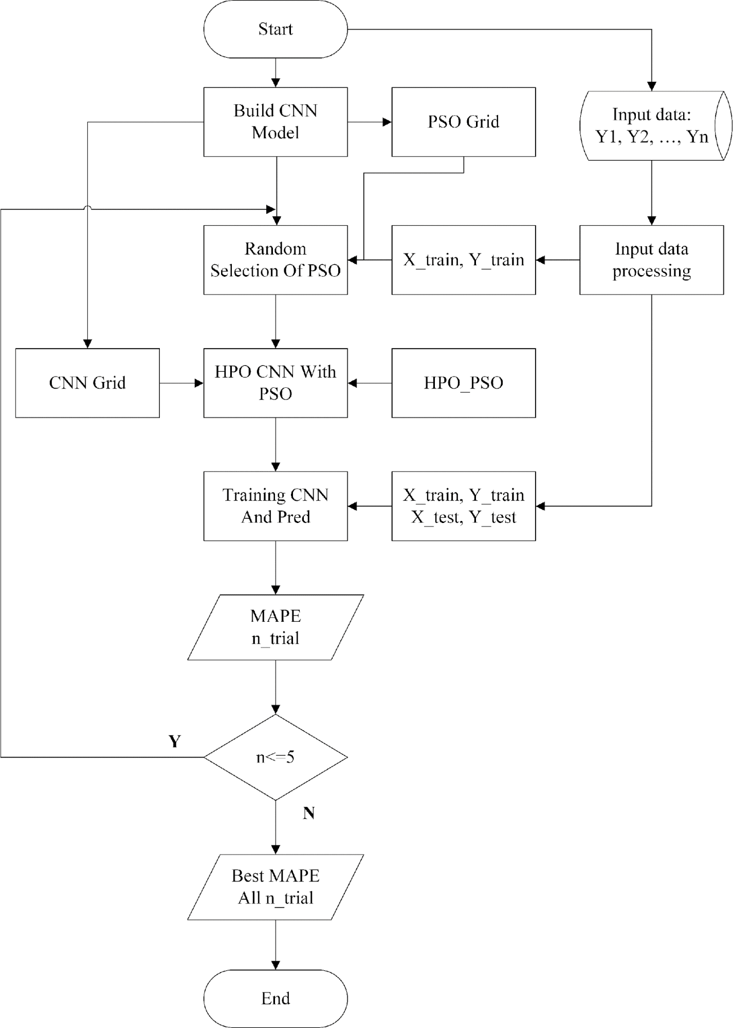
Figure 1. CNN–PSO Optimization Framework for Load Forecasting
RESULT AND DISCUSSION
Data
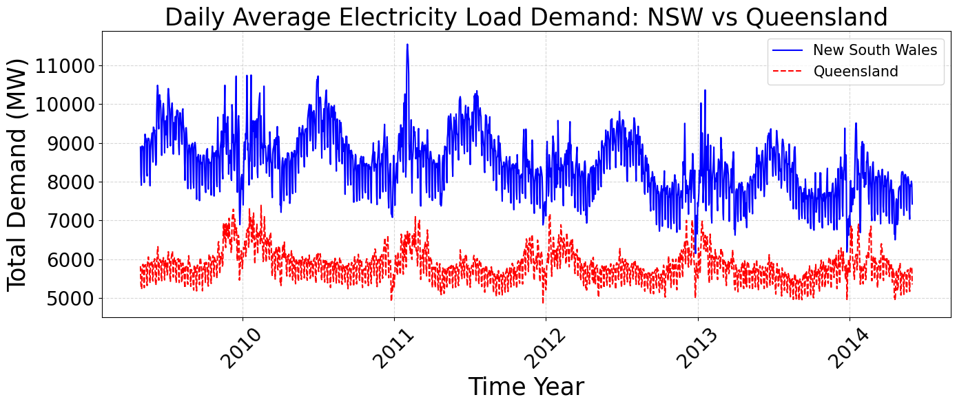
Figure 2 illustrates the daily average electricity load demand of New South Wales (NSW) and Queensland (QLD) from May 2009 to May 2014. The y-axis represents total demand in megawatts (MW), while the x-axis corresponds to time (in years). The NSW dataset shows significantly higher and more volatile demand levels than QLD. Both states exhibit clear seasonal cycles, with demand peaking during summer (due to air conditioning) and winter (due to heating). Notably, NSW features sharp spikes, especially during winter, indicating strong sensitivity to extreme temperatures or industrial activities. In contrast, QLD maintains a smoother and more stable profile throughout the period.
These characteristics provide contrasting data scenarios for evaluating the robustness of the proposed PSO–CNN framework. The NSW dataset’s volatility poses a greater modeling challenge, potentially requiring deeper networks and more extensive optimization, while QLD’s stability may yield satisfactory results with fewer iterations. Figure 3 presents the seasonal boxplot of daily average electricity demand in New South Wales (NSW) and Queensland (QLD) from 2009 to 2014. The Figure 3 shows that NSW consistently records higher and more volatile electricity consumption than QLD. Peak demand values are observed during summer and winter, corresponding to increased usage of cooling and heating systems. The broader interquartile range and more frequent outliers in NSW—especially in winter—reflect higher variability in daily load patterns. In contrast, QLD exhibits more stable seasonal behavior with less fluctuation. These differences highlight the necessity for adaptive hyperparameter optimization techniques, such as PSO, to improve forecasting accuracy under varying regional and seasonal load characteristics.
Figure 2. Daily Average Electricity Load Demand of NSW and QLD (May 2009 – May 2014)
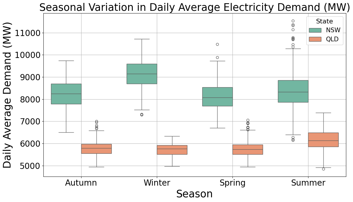
Figure 3. Seasonal Boxplot of Daily Average Electricity Load Demand in NSW and QLD (2009–2014)
Hyperparameter Grid
Table 1 summarizes the hyperparameter space for tuning the CNN model and PSO algorithm. For CNN, the number of filters in four convolutional layers is selected from {16, 32, 64, 128}, enabling flexible depth and feature complexity. Batch size values {16, 32, 64} balance computational cost and model stability, while training epochs {100–500} allow shallow and deeper training. For PSO, swarm size {1, 3, 5, 7, 9} and max iterations {2, 4, 6, 8, 10} define the search intensity and computational budget. Each trial randomly selects one pair, with total evaluations equal to their product. A 3-fold cross-validation strategy ensures robust evaluation, and Mean Absolute Percentage Error (MAPE) is the objective function. This structured setup supports efficient optimization and highlights how PSO configurations affect CNN performance in short-term load forecasting.
Table 1. Hyperparameter Space for CNN and PSO
Component | Parameter | Search Space / Value |
CNN Hyperparameter | Number of filters (filters_1 to filters_4) | {16, 32, 64, 128} |
CNN Hyperparameter | Batch size | {16, 32, 64} |
CNN Hyperparameter | Training epochs | {100, 200, 300, 400, 500} |
PSO Hyperparameter | Swarm size | {1, 3, 5, 7, 9} |
PSO Hyperparameter | Max iterations (maxiter) | {2, 4, 6, 8, 10} |
Evaluation Method | Cross-validation | 3-fold |
Objective Function | MAPE | Minimize |
Evaluation Outcomes
Figure 4 presents the convergence process of the Mean Absolute Percentage Error (MAPE) during the hyperparameter optimization of the CNN model using the Particle Swarm Optimization (PSO) algorithm on the New South Wales (NSW) dataset. The light blue line represents the MAPE values at each evaluation step, showing considerable fluctuations, especially during the early stages. However, the dashed dark blue line—representing the rolling mean with a window size of 10—indicates a stabilizing trend over time, decreasing variability in later stages. Notably, the red dashed-dotted line depicts the cumulative best MAPE achieved throughout the optimization process, which stabilizes very early (around the third evaluation), indicating that PSO quickly identified a near-optimal solution and maintained it consistently. This suggests that PSO demonstrated efficient convergence within the explored hyperparameter space. It highlights the potential influence of PSO settings, such as swarm size and iteration count, on its ability to effectively examine and refine optimal solutions.
Figure 5 presents the convergence behavior of the Mean Absolute Percentage Error (MAPE) during the CNN hyperparameter optimization process using the Particle Swarm Optimization (PSO) algorithm on the Queensland (QLD) dataset. The orange line represents individual MAPE values over each evaluation step, which display notable fluctuations throughout the process. The blue dashed line, representing a rolling average with a window size of 10, helps smooth these fluctuations and reveals a general stabilization trend, particularly in the later evaluation stages. The red dash-dot line indicates the cumulative best MAPE achieved, which remains consistently low from the early stages onward, suggesting that PSO was able to identify a good solution early and retain it.
Both Figure 4 and Figure 5 illustrate the effectiveness of PSO in locating optimal or near-optimal CNN hyperparameters within relatively few evaluations. However, the NSW dataset (Figure 4) exhibits slightly higher volatility in the initial MAPE values but achieves faster and more stable convergence. In contrast, the QLD dataset (Figure 5) shows more persistent oscillations in MAPE values across a broader range of evaluations, though convergence is ultimately achieved. Additionally, the cumulative best MAPE for QLD stabilizes at a slightly higher value than NSW, implying that the forecasting task for QLD might be somewhat more challenging or that the model was less sensitive to PSO hyperparameter variations. These differences may stem from the distinct demand characteristics and variability inherent in each region’s load profile, reinforcing the importance of adaptive optimization strategies tailored to the specific dataset.
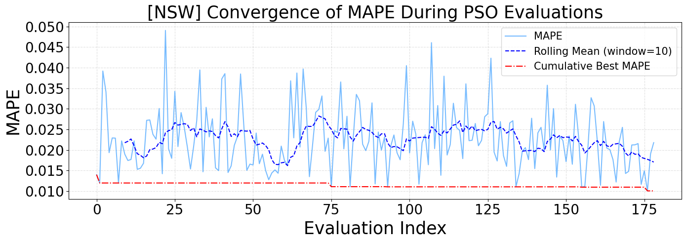
Figure 4. Convergence of MAPE During PSO Evaluations for NSW
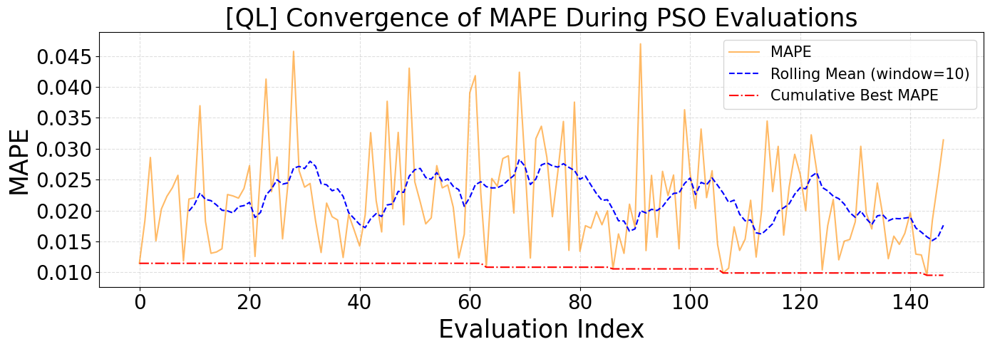
Figure 5. Convergence of MAPE During PSO Evaluations for QLD
Figure 6 illustrates the variability of the Mean Absolute Percentage Error (MAPE) across five runs of the Particle Swarm Optimization (PSO) algorithm for the state of New South Wales (NSW), with outliers removed based on the 1.5×IQR threshold to improve data representativeness. The results show that the median MAPE fluctuates slightly in the range of 0.020–0.022, with the lowest values observed in runs 2 and 3 (0.021). The first quartile (Q1) remains stable between 0.016 and 0.020, while the third quartile (Q3) varies from 0.023 to 0.029. Although the differences between PSO runs are not substantial, some runs exhibit a wider range of variation. Removing outliers has helped reduce variability and enhance the reliability of model performance evaluation. These results indicate a relatively good level of reproducibility of PSO when applied to highly fluctuating electricity load data in NSW.
Figure 7 illustrates the variability of the Mean Absolute Percentage Error (MAPE) across five runs of the Particle Swarm Optimization (PSO) algorithm for the state of Queensland (QLD), with outliers removed using the 1.5×IQR rule to enhance the robustness of the statistical summary. The median MAPE values range from 0.018 to 0.023, with run 5 achieving the lowest median (0.018). The first quartile (Q1) is relatively consistent, fluctuating between 0.014 and 0.020, while the third quartile (Q3) remains in the range of 0.022 to 0.027. These narrow interquartile ranges indicate a stable performance of PSO across multiple runs for QLD. Compared to Figure 6 (NSW), the QLD runs show slightly lower variability and tighter MAPE distributions, especially regarding Q1 and Q3 spread. NSW displays a wider IQR and higher Q3 values in some runs (up to 0.029), suggesting more pronounced fluctuations in model performance, likely due to NSW's more volatile electricity demand. Both states demonstrate reasonable PSO reproducibility, but QLD exhibits slightly more consistent optimization outcomes across runs.
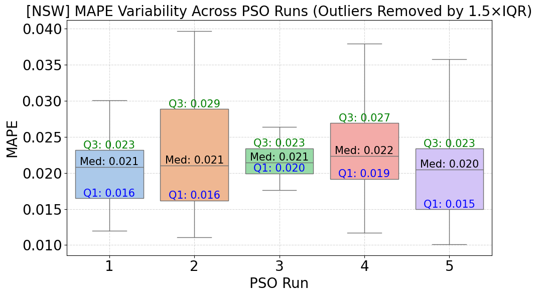
Figure 6. MAPE Distribution Across 5 PSO Runs – NSW Dataset
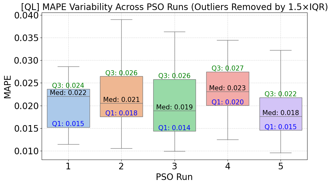
Figure 7. MAPE Distribution Across 5 PSO Runs – QLD Dataset
Figure 8 presents a heatmap of the average MAPE values obtained from different combinations of the PSO hyperparameters swarmsize and maxiter, applied to a CNN model using the dataset from New South Wales (NSW). The results clearly show that the combination (swarmsize = 5, maxiter = 8) achieves the lowest MAPE of 0.0202, indicating effective convergence with a small swarm size and a relatively high number of iterations. Conversely, reducing maxiter to 6 while keeping swarmsize = 5 leads to the highest MAPE of 0.0250, suggesting that increasing the number of iterations does not continually improve accuracy and may even result in premature convergence or overfitting. Moreover, configurations with smaller swarm sizes (5–7) generally perform better than larger ones. This underscores the importance of selecting appropriate PSO hyperparameters to optimize forecasting performance in complex, highly variable environments like NSW.
Figure 9 presents a heatmap of the average MAPE values corresponding to various swarm sizes and maxiter combinations when applying PSO to CNN training on the Queensland (QL) dataset. The best performance is achieved with the configuration (swarmsize = 5, maxiter = 4), yielding the lowest MAPE of 0.0187. In contrast, increasing the number of particles or iterations—such as (swarmsize = 7, maxiter = 8) and (swarmsize = 1, maxiter = 10)—results in higher MAPE values of 0.0232 and 0.0234, respectively. These findings indicate that simpler and faster PSO settings (lower maxiter, moderate swarmsize) are more effective for QLD's relatively stable load patterns. In comparison to Figure 8 (NSW), where the lowest MAPE (0.0202) is achieved at (swarmsize = 5, maxiter = 8), QLD benefits from a more minor iteration count. Furthermore, NSW experiences greater performance variation across configurations, suggesting that NSW’s more volatile load patterns require deeper exploration (higher maxiter), whereas QLD performs better with faster convergence. Overall, this emphasizes that PSO hyperparameter tuning must be tailored to regional characteristics to optimize forecasting accuracy effectively.
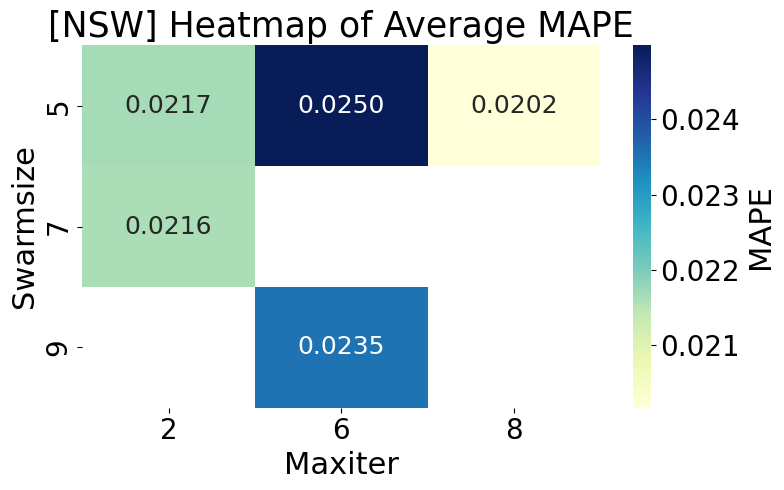
Figure 8. Heatmap of Average MAPE by swarmsize × maxiter – NSW Dataset
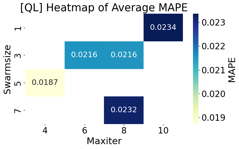
Figure 9. Heatmap of Average MAPE by swarmsize × maxiter – QLD Dataset
Discussion
The experimental findings across both the NSW and QLD datasets affirm that the configuration of Particle Swarm Optimization (PSO) parameters plays a critical role in influencing the forecasting performance of the CNN model. Although PSO-based hyperparameter tuning proved beneficial in both cases, noticeable differences emerged in convergence behavior and model stability. In particular, the NSW dataset, characterized by its highly volatile and irregular load patterns, resulted in more unstable optimization dynamics. This instability is evidenced by the broader interquartile ranges and wider dispersion of MAPE values shown in Figure 3 and Figure 5, even after outliers were removed. These results imply a higher sensitivity to initial parameter configurations and a greater risk of premature convergence or overfitting. The QLD dataset exhibited more stable convergence curves and consistent forecasting performance, as illustrated in Figure 4 and Figure 6. The relatively narrow IQRs and lower MAPE variability across multiple PSO runs suggest that the load characteristics in QLD are smoother and more predictable, thereby enabling PSO to converge more reliably to optimal solutions. The heatmaps presented in Figure 8 and Figure 9 further validate these findings. The optimal combination of PSO parameters differs between states. While QLD achieved its lowest MAPE (0.0187) with a smaller swarm size (5) and lower maxiter (4), NSW required a higher maxiter (8) under the same swarm size to reach its best performance (0.0202). These observations underscore the necessity of dataset-specific PSO tuning, especially when applying deep learning models to regions with distinct load volatility. These results demonstrate that PSO-CNN forecasting systems should not employ a one-size-fits-all configuration. Instead, they must be dynamically adjusted to account for the underlying variability in electricity demand patterns, as revealed by comparative analyses of both convergence trends and performance distributions.
CONCLUSIONS
This study proposed a PSO-based hyperparameter optimization framework to improve Convolutional Neural Networks (CNNs) forecasting accuracy in short-term electricity load forecasting. By systematically evaluating the influence of two critical PSO parameters—swarm size and maximum iterations—across multiple experimental runs, the study provides empirical evidence that careful tuning of PSO configurations can significantly enhance model performance, particularly when adapted to the characteristics of specific datasets. Using real-world datasets from New South Wales (NSW) and Queensland (QLD), the experimental results revealed that PSO's effectiveness is highly data-dependent. Specifically, the NSW dataset, characterized by greater load volatility and seasonal fluctuations, required higher iteration counts and moderate swarm sizes to achieve stable and accurate convergence. In contrast, with more consistent and smoother load behavior, the QLD dataset showed better performance with smaller swarm sizes and fewer iterations. These findings underscore a key theoretical contribution: there is no universally optimal PSO configuration, and data complexity and temporal patterns must guide hyperparameter tuning. This emphasizes the need for context-aware optimization strategies, particularly in dynamic environments like electricity load forecasting. Visual analyses using boxplots and convergence plots demonstrated varying MAPE dispersion, especially in the NSW case, while heatmap visualizations confirmed that suboptimal configurations can significantly degrade model performance. These results provide practical design guidelines for selecting PSO settings based on regional data behavior and computational constraints.
However, the study is subject to several limitations. First, the CNN architecture was fixed throughout all experiments, restricting the exploration of more profound, more complex, or alternative model structures. Second, the PSO search space was limited to a relatively small and discrete range of parameters (e.g., swarm size and iteration values), primarily for computational feasibility. While a fixed structure supports consistency in evaluating PSO parameter effects, it limits the generalizability of the findings to other model designs. Third, MAPE was the sole evaluation metric used, which may not fully reflect forecasting quality in periods with near-zero demand. Future studies should consider additional metrics like SMAPE and RMSE for a more comprehensive evaluation. Importantly, to ensure global search behavior and avoid overfitting in high-dimensional parameter spaces, a random sampling mechanism was integrated into the hyperparameter search process, prioritizing generalization and robustness over local optimization. This strategic choice helps maintain the integrity of the search results and provides a more realistic assessment of PSO's tuning capacity.
For future work, we recommend extending this framework in several directions. First, testing hybrid optimization strategies, such as combining PSO with Bayesian Optimization or Genetic Algorithms, may improve exploration–exploitation balance and convergence stability. Second, evaluating this framework on other deep learning architectures—including LSTM, Transformer models, or hybrid structures—could validate the generalizability of the findings. Third, applying the approach to multi-step forecasting tasks or across multiple regions may enhance its practical relevance. Finally, incorporating adaptive PSO schemes—where parameter values dynamically adjust during optimization—may provide superior performance across varying load profiles and time horizons. In summary, this study contributes theoretical and practical insights into integrating PSO and CNNs in short-term electricity load forecasting. It validates the importance of dataset-specific hyperparameter tuning and presents a replicable framework for guiding metaheuristic optimization in energy prediction tasks. Researchers and practitioners are encouraged to move beyond static or heuristic configurations and adopt adaptive optimization strategies that reflect the dynamic nature of power systems.
REFERENCES
- H. Mohd, P. Lazim, and P. Hajek, “An Optimized Hybrid Forecasting Model and Its Application to Air Pollution Concentration,” Arab. J. Sci. Eng., 2020, https://doi.org/10.1007/s13369-020-04572-w.
- M. Saviozzi, S. Massucco, and F. Silvestro, “Implementation of advanced functionalities for Distribution Management Systems: Load forecasting and modeling through Artificial Neural Networks ensembles,” Electr. Power Syst. Res., vol. 167, no. September 2018, pp. 230–239, 2019, https://doi.org/10.1016/j.epsr.2018.10.036.
- K. Yang, H. Wang, Q. Yang, Y. Shi, C. Zhu, and J. Bi, “An Ensemble Broad Learning Scheme for Short-Term Load Forecasting,” Proc. - 2022 Chinese Autom. Congr. CAC 2022, vol. 2022, pp. 4901–4905, 2022, https://doi.org/10.1109/CAC57257.2022.10056068.
- H. Oqaibi and J. Bedi, “A data decomposition and attention mechanism-based hybrid approach for electricity load forecasting,” Complex Intell. Syst., vol. 10, no. 3, pp. 4103–4118, 2024, https://doi.org/10.1007/s40747-024-01380-9.
- [5] M. Choubey, J. S. Yadav, and R. K. Chaurasiya, “Stacking Model for Short-Term Electrical Load Forecasting,” 2023 3rd Int. Conf. Energy, Power Electr. Eng. EPEE 2023, pp. 1285–1290, 2023, https://doi.org/10.1109/EPEE59859.2023.10351850.
- H. Liu, Y. Tang, Y. Pu, F. Mei, and D. Sidorov, “Short-term Load Forecasting of Multi-Energy in Integrated Energy System Based on Multivariate Phase Space Reconstruction and Support Vector Regression Model,” Electr. Power Syst. Res., vol. 210, no. April, p. 108066, 2022, https://doi.org/10.1016/j.epsr.2022.108066.
- A. Livas-García, O. May Tzuc, E. Cruz May, R. Tariq, M. Jimenez Torres, and A. Bassam, “Forecasting of locational marginal price components with artificial intelligence and sensitivity analysis: A study under tropical weather and renewable power for the Mexican Southeast,” Electr. Power Syst. Res., vol. 206, no. November 2021, p. 107793, 2022, https://doi.org/10.1016/j.epsr.2022.107793.
- O. Cagcag Yolcu, H. K. Lam, and U. Yolcu, “Short-term load forecasting: cascade intuitionistic fuzzy time series—univariate and bivariate models,” Neural Comput. Appl., vol. 5, 2024, https://doi.org/10.1007/s00521-024-10280-5.
- Z. Chen, T. Jin, X. Zheng, Y. Liu, Z. Zhuang, and M. A. Mohamed, “An innovative method-based CEEMDAN–IGWO–GRU hybrid algorithm for short-term load forecasting,” Electr. Eng., vol. 104, no. 5, pp. 3137–3156, 2022, https://doi.org/10.1007/s00202-022-01533-4.
- S. K. Panda and P. Ray, “An Effect of Machine Learning Techniques in Electrical Load forecasting and Optimization of Renewable Energy Sources,” J. Inst. Eng. Ser. B, vol. 103, no. 3, pp. 721–736, 2022, https://doi.org/10.1007/s40031-021-00688-1.
- W. Khan, W. Somers, S. Walker, K. de Bont, J. Van der Velden, and W. Zeiler, “Comparison of electric vehicle load forecasting across different spatial levels with incorporated uncertainty estimation,” Energy, vol. 283, no. February, p. 129213, 2023, https://doi.org/10.1016/j.energy.2023.129213.
- Z. Liao, H. Pan, and X. Fan, “Multiple Wavelet Convolutional Neural Network for Short-Term Load Forecasting,” vol. 8, no. 12, pp. 9730–9739, 2021, https://doi.org/10.1109/JIOT.2020.3026733.
- F. C. de Lima Duarte, P. S. G. de Mattos Neto, and P. R. A. Firmino, “A hybrid recursive direct system for multi-step mortality rate forecasting,” J. Supercomput., vol. 80, no. 13, pp. 18430–18463, 2024, https://doi.org/10.1007/s11227-024-06182-x.
- A. Ghasemieh, A. Lloyed, P. Bahrami, P. Vajar, and R. Kashef, “A novel machine learning model with Stacking Ensemble Learner for predicting emergency readmission of heart-disease patients,” Decis. Anal. J., vol. 7, no. May, p. 100242, 2023, https://doi.org/10.1016/j.dajour.2023.100242.
- G. F. Fan et al., “A new intelligent hybrid forecasting method for power load considering uncertainty,” Knowledge-Based Syst., vol. 280, no. 58, p. 111034, 2023, https://doi.org/10.1016/j.knosys.2023.111034.
- J. Wang and J. Cao, “Deep Learning Reservoir Porosity Prediction Using Integrated Neural Network,” Arab. J. Sci. Eng., no. 0123456789, 2021, https://doi.org/10.1007/s13369-021-06080-x .
- T. Nguyen Da, M. Y. Cho, and P. Nguyen Thanh, “Optimizing K-means clustering center selection with density-based spatial cluster in radial basis function neural network for load forecasting of smart solar microgrid,” Electr. Eng., pp. 1-16, 2024, https://doi.org/10.1007/s00202-024-02599-y.
- Z. Sheng, H. Wang, G. Chen, B. Zhou, and J. Sun, “Convolutional residual network to short-term load forecasting,” Appl. Intell., vol. 51, no. 4, pp. 2485–2499, 2021, https://doi.org/10.1007/s10489-020-01932-9.
- X. Chen, M. Yang, Y. Zhang, J. Liu, and S. Yin, “Load Prediction Model of Integrated Energy System Based on CNN-LSTM,” 2023 3rd Int. Conf. Energy Eng. Power Syst. EEPS 2023, pp. 248–251, 2023, https://doi.org/10.1109/EEPS58791.2023.10257124.
- Y. Li, Y. Ye, Y. Xu, L. Li, X. Chen, and J. Huang, “Two-stage forecasting of TCN-GRU short-term load considering error compensation and real-time decomposition,” Earth Sci. Informatics, vol. 17, no. 6, pp. 5347-5357, 2024, https://doi.org/10.1007/s12145-024-01456-7.
- C. Tong, L. Zhang, H. Li, and Y. Ding, “Attention-based temporal–spatial convolutional network for ultra-short-term load forecasting,” Electr. Power Syst. Res., vol. 220, no. December 2022, p. 109329, 2023, https://doi.org/10.1016/j.epsr.2023.109329.
- N. M. M. Bendaoud, N. Farah, and S. Ben Ahmed, “Applying load profiles propagation to machine learning based electrical energy forecasting,” Electr. Power Syst. Res., vol. 203, no. October 2021, p. 107635, 2022, https://doi.org/10.1016/j.epsr.2021.107635.
- R. Keshvari, M. Imani, and M. Parsa Moghaddam, “A clustering-based short-term load forecasting using independent component analysis and multi-scale decomposition transform,” J. Supercomput., vol. 78, no. 6, pp. 7908–7935, 2022, https://doi.org/10.1007/s11227-021-04195-4.
- S. Yin, Z. Chen, W. Liu, and Z. Su, “Ultra short term charging load forecasting based on improved data decomposition and hybrid neural network,” IEEE Access, vol. 13, no. April, pp. 58778–58789, 2025, https://doi.org/10.1109/ACCESS.2025.3555737.
- G. Tricarico, F. Gonzalez-Longatt, F. Marasciuolo, O. Ishchenko, M. Dicorato, and G. Forte, “Sizing and Siting of Energy Storage Systems for Mitigating Forecast Mismatch in Transmission Grid,” IEEE Trans. Ind. Appl., vol. 61, no. 1, pp. 1–12, 2025, https://doi.org/10.1109/TIA.2025.3532580.
- B. Li, Y. Mo, F. Gao, and X. Bai, “Short-term probabilistic load forecasting method based on uncertainty estimation and deep learning model considering meteorological factors,” Electr. Power Syst. Res., vol. 225, no. August, p. 109804, 2023, https://doi.org/10.1016/j.epsr.2023.109804.
- Y. R. K. Teeparthi, “Distribution System State Estimation with Convolutional Generative Adversarial Imputation Networks for Missing Measurement Data,” Arab. J. Sci. Eng., 2023, https://doi.org/10.1007/s13369-023-08393-5.
- Y. K. Ahranjani, M. Beiraghi, and R. Ghanizadeh, “Short time load forecasting for Urmia city using the novel CNN-LTSM deep learning structure,” Electr. Eng., 2024, https://doi.org/10.1007/s00202-024-02361-4.
- O. Rubasinghe, X. Zhang, T. K. Chau, Y. H. Chow, T. Fernando, and H. H. C. Iu, “A Novel Sequence to Sequence Data Modelling Based CNN-LSTM Algorithm for Three Years Ahead Monthly Peak Load Forecasting,” IEEE Trans. Power Syst., vol. 39, no. 1, pp. 1932–1947, 2024, https://doi.org/10.1109/TPWRS.2023.3271325.
- Y. Guo, J. Wang, Y. Zhong, T. Wang, and Z. Sui, “A Novel Electrical Load Forecasting Model for Extreme Weather Events Based on Improved Gated Spiking Neural P Systems and Frequency Enhanced Channel Attention Mechanism,” IEEE Access, vol. 13, no. November 2024, pp. 4884–4911, 2025, https://doi.org/10.1109/ACCESS.2025.3525479.
- Z. Lin, L. Xie, and S. Zhang, “A compound framework for short-term gas load forecasting combining time-enhanced perception transformer and two-stage feature extraction,” Energy, vol. 298, no. April, p. 131365, 2024, https://doi.org/10.1016/j.energy.2024.131365.
- C. Wei, D. Pi, M. Ping, and H. Zhang, “Short-term load forecasting using spatial-temporal embedding graph neural network,” Electr. Power Syst. Res., vol. 225, no. August, p. 109873, 2023, https://doi.org/10.1016/j.epsr.2023.109873.
- B. Chen and Y. Wang, “Short-Term Electric Load Forecasting of Integrated Energy System Considering Nonlinear Synergy between Different Loads,” IEEE Access, vol. 9, pp. 43562–43573, 2021, https://doi.org/10.1109/ACCESS.2021.3066915.
- V. K. Saini, R. Kumar, A. S. Al-Sumaiti, A. Sujil, and E. Heydarian-Forushani, “Learning based short term wind speed forecasting models for smart grid applications: An extensive review and case study,” Electr. Power Syst. Res., vol. 222, no. May, p. 109502, 2023, https://doi.org/10.1016/j.epsr.2023.109502.
- T. Bashir, H. Wang, M. Tahir, and Y. Zhang, “Wind and solar power forecasting based on hybrid CNN-ABiLSTM, CNN-transformer-MLP models,” Renew. Energy, vol. 239, no. August 2024, p. 122055, 2025, https://doi.org/10.1016/j.renene.2024.122055.
- B. Mechanism, J. Xiao, P. Liu, H. Fang, and X. Liu, “Short-Term Residential Load Forecasting With Baseline-Refinement Profiles and,” IEEE Trans. Smart Grid, vol. 15, no. 1, pp. 1052–1062, 2024, https://doi.org/10.1109/TSG.2023.3290598.
- R. Lu et al., “A Novel Sequence-to-Sequence-Based Deep Learning Model for Multistep Load Forecasting,” IEEE Trans. Neural Networks Learn. Syst., vol. 36, no. 1, pp. 638–652, 2024, https://doi.org/10.1109/TNNLS.2023.3329466.
- F. Gao, J. Song, and X. Shao, “Short-term interval-valued load forecasting with a combined strategy of iHW and multioutput machine learning,” Ann. Oper. Res., vol. 346, no. 3, pp. 2009–2033, 2025, https://doi.org/10.1007/s10479-024-06446-y.
- N. A. Nguyen, T. D. Dang, E. Verdú, and V. Kumar Solanki, “Short-term forecasting electricity load by long short-term memory and reinforcement learning for optimization of hyper-parameters,” Evol. Intell., vol. 16, no. 5, pp. 1729–1746, 2023, https://doi.org/10.1007/s12065-023-00869-5.
- X. Wang, “Short-term Power Load Forecasting Model Based on Model Fusion,” pp. 141–144, 2020, https://doi.org/10.1109/AIAM50918.2020.00035.
- Y. Huang, Y. Zhao, Z. Wang, X. Liu, and Y. Fu, “Sparse dynamic graph learning for district heat load forecasting,” Appl. Energy, vol. 371, no. March, p. 123685, 2024, https://doi.org/10.1016/j.apenergy.2024.123685.
- D. Kiruthiga and V. Manikandan, “Levy flight-particle swarm optimization-assisted BiLSTM + dropout deep learning model for short-term load forecasting,” Neural Comput. Appl., vol. 35, no. 3, pp. 2679–2700, 2023, https://doi.org/10.1007/s00521-022-07751-y.
- X. T. Luong, V. H. Bui, D. T. Do, T. H. Quach, and V. A. Truong, “An Improvement of Maximum Power Point Tracking Algorithm Based on Particle Swarm Optimization Method for Photovoltaic System,” Proc. 2020 5th Int. Conf. Green Technol. Sustain. Dev. GTSD 2020, no. November, pp. 53–58, 2020, https://doi.org/10.1109/GTSD50082.2020.9303110.
- M. Pratap, Y. Rohit, and D. Kumar, “Resource Provisioning Through Machine Learning in Cloud Services,” Arab. J. Sci. Eng., 2021, https://doi.org/10.1007/s13369-021-05864-5.
- W. Liu et al., “Short-term load forecasting based on elastic net improved GMDH and difference degree weighting optimizations,” Appl. Sci., vol. 8, no. 9, 2018, https://doi.org/10.3390/app8091603.
- T. A. Nguyen and T. N. Tran, “Improving Short-Term Electrical Load Forecasting with Dilated Convolutional Neural Networks: A Comparative Analysis,” J. Robot. Control, vol. 6, no. 2, pp. 560–569, 2025, https://doi.org/10.18196/jrc.v6i2.24967.
AUTHOR BIOGRAPHY

| Nguyen Anh Tuan     received a B.Sc. degree from the Industrial University of Ho Chi Minh City, Vietnam 2012, and an M.Sc. degree from the HCMC University of Technology and Education, Vietnam, in 2015. He is a Lecturer with the Faculty of Electrical Engineering Technology at the Industrial University of Ho Chi Minh City, Vietnam. His main research interests include power quality and load forecasting. received a B.Sc. degree from the Industrial University of Ho Chi Minh City, Vietnam 2012, and an M.Sc. degree from the HCMC University of Technology and Education, Vietnam, in 2015. He is a Lecturer with the Faculty of Electrical Engineering Technology at the Industrial University of Ho Chi Minh City, Vietnam. His main research interests include power quality and load forecasting. Email: nguyenanhtuan@iuh.edu.vn |
|
|

| Trung Dung Nguyen was born in 1976 in Vietnam. He received a Master’s degree in Electrical Engineering from Ho Chi Minh City University of Technology and Education, Vietnam, in 2017. He lectures at the Faculty of Electrical Engineering Technology, Industrial University of Ho Chi Minh City, Ho Chi Minh City, Vietnam. His research focuses on applications of metaheuristic algorithms in power system optimization, optimal control, and model predictive control. Email: nguyentrungdung@iuh.edu.vn
|
Tuan Anh Nguyen (Analysis of Swarm Size and Iteration Count in Particle Swarm Optimization for Convolutional Neural Network Hyperparameter Optimization in Short-Term Load Forecasting)