Sensor Fusion of Laser and Inertial Units with Kalman-KMeans-Fuzzy Framework for Real-Time Railway Geometry Monitoring

Ahmad Atif Fikri, Muhammad Ferindin Nuha Subhan, Heru Suryanto, Krisna Dwipa Muhdi,

Daniel Febrian Pratama, Ahmad Iqbal

Mechanical Engineering Study Program, Universitas Negeri Malang, Semarang Street No.5, Malang City, Indonesia

1. INTRODUCTION

Railways remain a critical mode of global mobility and trade, offering an efficient and environmentally sustainable means of transporting people and goods over long distances. However, the safety and integrity of railway infrastructure are paramount, with track maintenance playing a vital role in ensuring uninterrupted and secure train operations. Among the most significant risks to rail safety is derailment, which can result in severe economic losses, environmental hazards, and human casualties. For instance, a case of track damage resulting from height differences. Understanding derailment statistics, causes, and consequences is essential for implementing effective prevention strategies [30].

Derailments are a persistent global issue. In the United States, As reported an average of 400 derailments annually over a span of 17 years [30]. According to the Federal Railroad Administration (FRA), this translates to approximately 1.85 derailments per million train-miles. Canada reports a slightly lower rate of 1.7 derailments per million train-miles. In contrast, countries such as Germany have achieved even lower rates (0.7 per million train-miles), reflecting disparities in infrastructure investment and monitoring technology [31]. These incidents cause service disruptions and impose heavy financial and operational burdens, further emphasizing the need for proactive monitoring systems. Human factors such as operator error and design flaws are also leading contributors to derailments. Between 1980 and 2019, railway accidents across Europe were largely attributed to collisions, derailments, and incidents at crossings, underscoring the persistent nature of this problem [51]. Derailments are caused by multiple interrelated factors, including human error, infrastructure faults, and rolling stock failures. Inadequately designed railway systems amplify human error risks [52]. Track irregularities such as buckling, misalignment, and rail damage are frequently cited as precursors to derailments [53][54]. Coupler failures are also a major concern; Appoh and Yunusa-Kaltungo reported 133 derailments involving over 770 railcars in the U.S. due to such failures [55]. Equipment malfunctions, such as overheated axle boxes (hot boxes), contribute to approximately 5% of derailments [59]. Environmental influences such as extreme weather further compound these risks. Rungskunroch highlighted how weather extremes degrade infrastructure resilience and increase the likelihood of derailments [74]. Likewise, [81] and [82] emphasized that natural disasters compromise track integrity, calling for a comprehensive risk management strategy.

The economic consequences of derailments extend far beyond immediate repair costs. Significant expenditures are often associated with infrastructure damage and environmental contamination especially when hazardous materials (HAZMAT) are involved [52]. Lim and Kim demonstrated the considerable financial losses tied to weather-induced railway accidents [83]. Reports estimate that derailment-related service disruptions can lead to revenue losses between USD 10,000 and 25,000 per hour, depending on the corridor and cargo type [84]. Dangerous goods incidents also result in higher insurance premiums and liability costs [85]. Over time, such events can inflict reputational damage and erode public confidence in rail systems [86]. Therefore, workforce training and modern monitoring technologies are essential elements of any effective prevention strategy [87]. Advanced forecasting models, like those proposed by Lim and Kim, offer valuable tools for optimizing infrastructure investments and improving economic resilience [93].

Derailments also result in serious human and environmental consequences. In India alone, 17,993 rail accidents in 2021 led to 16,431 fatalities and 1,852 injuries. Esmaeeli emphasized the importance of individualized risk assessments to estimate potential casualties [52]. Beyond physical harm, the psychological impact on survivors and witnesses is an underexplored area. Environmentally, derailments involving HAZMAT can be disastrous. The 2023 East Palestine, Ohio derailment, in which vinyl chloride and other hazardous chemicals were released, required mass evacuations and raised long-term public health concerns [95]. Toxic spills can cause long-term damage to land, water, and biodiversity, highlighting the need for robust emergency preparedness frameworks [97].

Conventional manual inspection methods remain widely used but are increasingly inadequate for modern railway networks. These techniques are time-intensive, labor-dependent, and reliant on subjective human interpretation. Visual inspections are prone to human error and inconsistency due to variability in inspector expertise [52],[98]. Large-scale networks make full manual inspections impractical due to time and physical constraints [99], and limited inspection windows hinder comprehensive assessments [100]. Adverse weather further delays or compromises inspections [101]. Moreover, traditional methods have high false-negative rates and lack the frequency to detect problems before they escalate [102]. In most railway networks, manual inspections are typically performed at monthly or biweekly intervals, which limits the ability to detect rapidly emerging defects and compromises the timeliness of maintenance interventions [100]. To address these limitations, sensor technologies have emerged as effective solutions for real-time track geometry monitoring. Table 1 provides a comparative analysis of common sensor types, outlining their performance advantages and limitations. Among them, the VL53L0X laser and MPU6050 Inertial Measurement Unit (IMU) sensors were selected for this study due to their favorable balance of precision, real-time capability, and cost-efficiency.

Based on this comparison, the integration of VL53L0X and MPU6050 sensors offers an optimal trade-off between cost, scalability, and functional performance, forming the basis for the proposed railway monitoring platform in this study. However, to date, no existing railway geometry monitoring system simultaneously offers real-time accuracy, scalability, and cost-effectiveness through an integrated sensor fusion framework [1][2]. The research contribution is for advancing intelligent, condition-based railway maintenance through the integration of multi-modal sensor technologies for real-time track geometry monitoring. The proposed system combines laser infrared sensors and an IMU mounted on a modular mobile platform to measure track gauge, height, and inclination with high precision [3]. By employing Kalman filtering for signal denoising, K-Means clustering for anomaly detection, and fuzzy logic for decision support, the system transforms raw measurement data into actionable maintenance insights. Experimental results demonstrate a substantial reduction in measurement noise, achieving Root Mean Square Error (RMSE) and Mean Absolute Error (MAE) values of 0.8165 mm and 0.3175 mm for width and height, and 0.3086° and 0.0952° for inclination, respectively. This integrated approach not only mitigates the limitations of manual inspections, such as low frequency and operator bias, but also offers a scalable, low-cost, and data-driven solution aligned with modern railway infrastructure management strategies. The platform paves the way for predictive maintenance models and digital twin applications, marking a shift toward proactive, efficient, and safer rail operations.

Table 1. Comparative Analysis of Sensor Technologies for Railway Track Geometry Monitoring

2. METHODS

This section describes the sensor characteristics, data acquisition hardware, post processing algorithms, experimental arrangement, and validation metrics employed in this work. The aim is to offer a detailed, clear description of the procedure that has led to the design and testing of the integrated sensor system for railway track geometry monitoring.

1. System Design, Overview and Sensors Calibration

The developed integrated sensor system in this study is aimed at overcoming the limitations of the conventional manual track inspection, taking fully real-time measured data with the benefits of automating, high-accuracy measurement and frequent monitoring of critical geometry parameters of the track. The sensor system is modular by design, combining several sensor technologies for a broad range of the data available. This multi-sensor strategy increases redundancy, and reliability in the system of sensors is enhanced, contributing to sound design methodology for integrated sensor systems in railway track geometry measurement [32]. The wiring schematic of the sensors through the data acquisition system is illustrated in Figure 1. It consists of the following major components:

• Sensors: The VL53L0X laser infrared sensor is used for non-contact measurement of track gauge and height. This sensor was selected due to its ability to quickly detect distances in both dynamic and static conditions, with an absolute measurement range of up to 2 meters across surfaces of varying colours. It is capable of real-time object detection at rates up to 50 Hz (i.e., every 20 ms), while maintaining low power consumption and offering cost-effective performance.
• Inclination is measured using the MPU6050 Inertial Measurement Unit (IMU). This sensor was chosen for its affordability and ability to detect motion and orientation. The MPU6050 is an integrated 6-axis IMU that combines a 3-axis MEMS accelerometer (±8 g) and a 3-axis MEMS gyroscope (±2000°/s), making it suitable for real-time dynamic monitoring. It operates with a typical current draw of 3.8 mA and demonstrates stable performance across a broad temperature range (−40 °C to +85 °C). Furthermore, it supports high-speed communication via the I²C interface, with data transfer rates up to 400 kHz. The MPU6050 remains a widely adopted motion-tracking sensor in applications demanding low power, low cost, and high reliability, particularly in wearable and mobile systems.
• Data Acquisition (DAQ) Unit: Although a separate DAQ system is not utilized, the data acquisition process is handled internally by the sensors. The VL53L0X includes an integrated Time-of-Flight (ToF) ranging engine that transmits processed distance data via I²C. Similarly, the MPU6050 features built-in Analog to Digital Converter (ADC), digital low-pass filters, and a FIFO buffer, enabling direct digital output. These embedded DAQ capabilities reduce hardware complexity and facilitate seamless data transmission to the processing unit.
• Processing Unit: The central processing core is led by an Arduino MEGA2560, which undertakes real-time data fusion and algorithmic computations. This unit processes raw sensor data utilizing a Kalman Filter for effective noise reduction, employs clustering techniques through the K-Means algorithm, and implements fuzzy logic for informed decision-making support in maintenance contexts. The Arduino MEGA2560 is characterized by extended memory and enhanced processing capabilities, rendering it adept at managing multiple sensor inputs and complex algorithmic functions with minimal latency.
• Output/Storage: Storage for data Secure Digital card (SD card) and a communication interface Universal Serial Bus (USB) data transfer and potentially real-time monitoring.

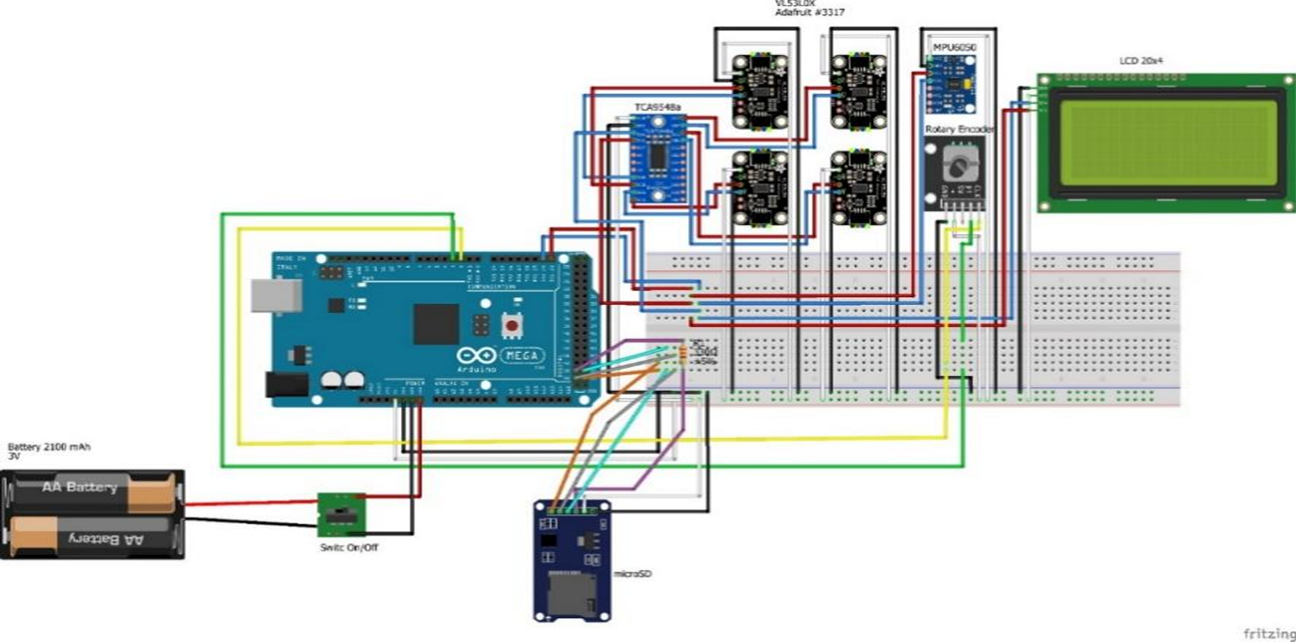
Figure 1. Wiring Diagram of Sensor Integration

Figure 2 is illustrates the physical implementation of the railway geometry monitoring system mounted on a custom-designed inspection trolley. The trolley is constructed for manual guidance along the rail, facilitating reliable sensor attachment that ensures precision in data collection over irregular surfaces. The system is developed based on mobility and terrain adaptability [33][34]. The trolley has a four-wheel design with adjustable wheel spacing. Finite element analysis has been shown in previous studies [35] to be effective in validating design rigidity and load-bearing capacity. While FEA was not performed in this study, its relevance supports the structural reasoning behind the trolley’s rigid frame design. The sensors are installed in a rigid frame, mounted on the trolley, and equipped with adjustable brackets for correct alignment and to prevent vibrations [37]. Figure 3 shows the procedure for each sensor, such as laser distance measurement sensors, IMU inclination sensor, and the actual arrangement of sensors on the inspection trolley. The consideration of sensor integration is for precise and efficient data acquisition [38]. The DAQ and basic signal processing functionalities are embedded within the sensors themselves. The VL53L0X infrared sensor integrates a Time-of-Flight ranging engine and communicates via I2C, while the MPU6050 includes onboard ADCs, low-pass filters, and a FIFO buffer for motion data acquisition. These sensors transmit raw data directly to the Arduino MEGA2560 processing unit, which is enclosed in a protective cover mounted on the trolley to shield it from environmental conditions, whereas the sensors remain exposed for unobstructed measurement.

To provide a clear overview of the data processing architecture and analytical framework employed in this study, a methodological flowchart is presented in Figure 3. This diagram illustrates the sequential stages starting from sensor installation and data acquisition, followed by Kalman-based noise filtering, unsupervised K-Means clustering for condition classification, and fuzzy logic-based decision support. The system then outputs maintenance recommendations, stores the processed information, and undergoes a final performance evaluation using standard metrics such as RMSE, MAE, F1-score, confusion matrix, and F-statistics [4]. This flow ensures traceability, modularity, and clarity in the execution of each computational and hardware step.

Figure 2. Field-Deployed Railway Geometry Monitoring Trolley with Integrated Laser and IMU Sensors

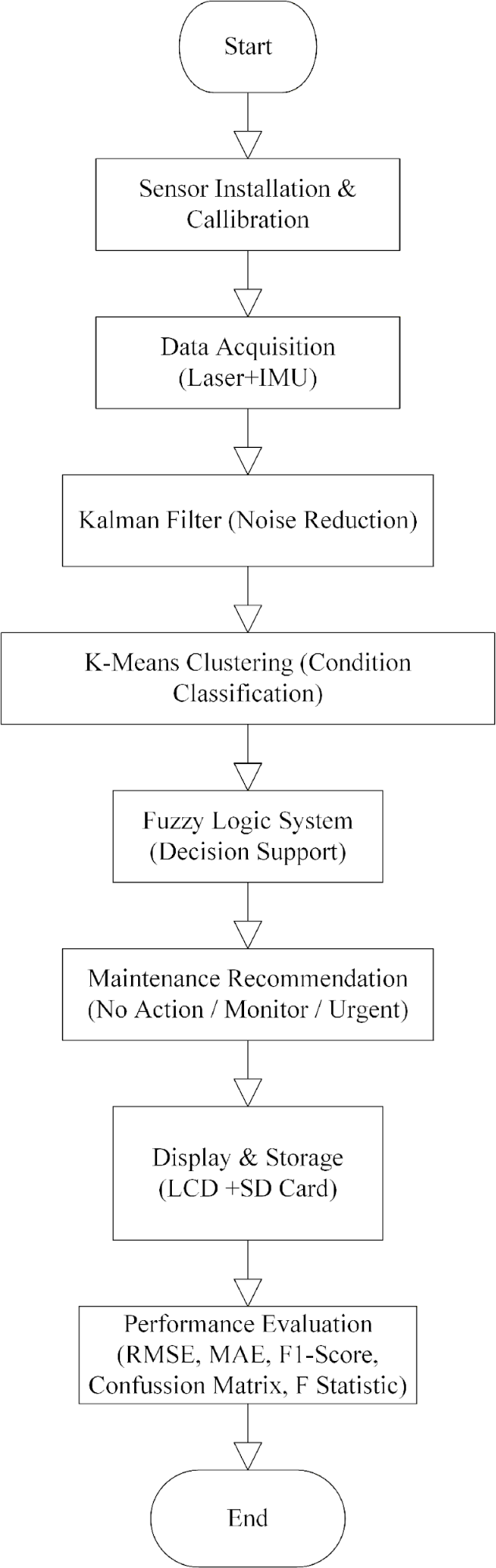
Figure 3. Methodological Flowchart

2. Sensor Calibration

Figure 4 illustrates the instrumentation setup used for sensor calibration and measurement testing, where a = 985 mm and b = 70 mm denote the respective offsets used in width and height calculations. The system comprises three primary sensor types: the VL53L0X laser infrared sensor for measuring both track gauge and height, and the MPU6050 IMU for inclination measurement. Calibration procedures were conducted under controlled conditions (20 ± 2 °C and 45–55% Relative Humidity (RH)) to ensure consistency and traceability [36]. Three types of sensors were employed in this study:

1. Track Gauge (Width) Sensor

Track gauge was measured using the VL53L0X time-of-flight laser-ranging sensor. The sensor was calibrated using certified reference jigs with known distances. It was securely mounted on a rigid base to minimize external vibration and ensure repeatability. The gauge calibration demonstrated high linearity with a maximum absolute error of ±0.05 mm and an R² value of 0.9998. The combined readings from the left and right sensors were processed using a constant offset (a = 985 mm) to compute the total gauge width (L).

2. Track Height Sensor

The same model of laser sensor VL53L0X was utilized for measuring track height. Calibration followed a similar procedure, using a reference jig with known height differences. The resulting calibration curve demonstrated a maximum relative error of ±0.06 mm and an  value of 0.9997. This procedure ensured consistent sensor performance under controlled environmental conditions. It is worth noting that simulation methods are often used to validate the mechanical response of such systems, especially under varying strain rates and springback conditions [40]. Data result of the height measurements from the left and right sides, using the same sensors, are each summed with a constant , resulting in the left-side height  and the right-side height .

3. Inclination (Cross-Level/Cant) Sensor

Inclination was measured using the MPU6050 Inertial Measurement Unit (IMU), combining a 3-axis accelerometer and a 3-axis gyroscope. Calibration was performed using a high-precision goniometer following manufacturer guidelines. The IMU was rotated across known angle increments, and output data were recorded to establish a calibration curve. Results indicated a maximum angular error of ±0.003°, confirming the sensor’s high fidelity in detecting angular deviations.

The laser infrared sensors were calibrated, according to best practice, for the measurement of the track geometry of the railway. This entailed precalibration preparation by firmly fixating the sensors and regulating environmental conditions [41][42]. The first calibration procedures were focused on making controls with reference objects (precision spheres) in such a way that they defined the reference measurements and that the zeroing point of the sensor output was defined [43]. Linear and angle calibrations were carried out and dynamic calibration was considered due to the movable nature of the platform [22],[44][45]. The infrared sensors were calibrated using a flat reference surface at known distances between 50–200 mm. Measured values were compared to ground truth to construct a linear fit curve ( = 0.9997), with a maximum absolute error of ±0.06 mm. The inclination sensor (MPU6050) was calibrated by aligning the device at known tilt angles and verifying the resulting angle computation from accelerometer readings. Observed deviations were minimal, with repeatable measurements within ±1.5°. The calibration approach was designed to align with traceability principles outlined in ISO 10360-10:2021 [5], which defines acceptance and verification procedures for laser-based dimensional measurement systems. Similarly, the IMU/inclinometer calibration was guided by general criteria from IEEE Standard 2700-2017 [6], which establishes performance metrics for MEMS-based inertial sensors. Measurement uncertainty was estimated based on the conceptual framework presented in Refs [46][47], considering key environmental and instrumental factors relevant to low-cost infrared sensing systems. Potential error sources and drift, as calibration, environmental conditions, optical path change, vibrations, and signal noise are recognised and counteracted with regular calibration, environmental control, novel sensor housing, vibration isolation, advanced signal treatment and feedback mechanisms [43][49]. Field validation was implemented according to best practice guidelines, including stable sensor mounting, ground-truth-based calibration under controlled environmental conditions, use of filtering techniques to reduce noise, and field-level testing with integrated multisensor data logging. While full industrial protocols were not adopted, the system design and validation methodology were aligned with core principles of traceable and repeatable sensor deployment [103],[50].

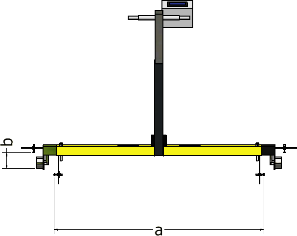
Figure 1. Sensor Measurement Test Equipment, a= 985 mm, b= 70 mm

3. Data Acquisition (DAQ) and Hardware Implementation

The DAQ system used in this work is managed using the internal capabilities of each sensor module, enabling lightweight integration and power efficiency suited for embedded platforms such as laser-based distance sensors and IMU MPU6050. The sensor fusion comprises a laser-based distance sensor (VL53L0X) and an Inertial Measurement Unit (IMU, MPU6050). Each sensor includes an internal data acquisition pipeline and communicates via I²C to the microcontroller.

1. Internal DAQ and Sampling Rate of VL53L0X

The VL53L0X is a time-of-flight (ToF) laser distance sensor capable of absolute distance measurements up to 2 meters. Its internal DAQ pipeline includes a Vertical-Cavity Surface-Emitting Laser (VCSEL) emitter, Single Photon Avalanche Diode (SPAD) photon detector array, and a ToF ranging engine, which performs signal acquisition and processing to calculate distance values. Although the VL53L0X sensors support high-frequency acquisition (up to 50 Hz and 500 Hz respectively), a fixed sampling interval of 0.5 seconds (2 Hz) was selected in this study. This data acquisition rate was determined empirically based on the trolley’s traversal speed, which followed an average human walking pace (~0.5–1 m/s), and the spatial resolution required for structural profiling. Manual reference measurements were taken every 0.5 meters along a 10-meter linear path to validate the system’s sensor outputs. Additionally, slower sampling helped suppress high-frequency measurement noise, avoid sensor over-triggering due to mechanical vibration, and simplify data processing on the embedded microcontroller [7]. This decision balances spatial resolution, noise control, and system responsiveness, making it suitable for real-time low-cost railway monitoring [8].

2. Integrated IMU DAQ Pipeline of MPU6050

The MPU6050 integrates a 3-axis accelerometer and 3-axis gyroscope, with internal 16-bit ADCs, low-pass filtering, and an optional Digital Motion Processor (DMP). The device supports configurable output rates from 10 Hz up to 500 Hz, and includes a 1024-byte FIFO buffer for burst-mode acquisition. For this study, a sampling rate of 2 Hz was selected as a balance between resolution and processing load [9]. This enables detection of rotational and lateral dynamics relevant to rail inclination and cross-level deviation at high spatial fidelity [8].

3. System Integration and Synchronization

Both sensors interface via I2C protocol to the Arduino Mega2560 [10]. A timestamp-based software synchronization scheme was used to align IMU and laser readings during acquisition cycles [11]. This design avoids reliance on external DAQ systems and allows real-time fusion and onboard processing (e.g., Kalman filtering) without significant latency. The system requires approximately 290 milliseconds to process and log each sensor fusion cycle such as KF, Clustering, and Fuzzy Inference. Power is supplied via a 5V battery module with regulated output to the sensor array. Data is stored to an SD card and transmitted via USB for offline analysis. The entire system is mounted on a custom-built aluminum trolley with adjustable sensor brackets and vibration-damped suspension to reduce motion artifacts during traversal.

4. Data Processing Algorithms

1. Kalman Filter Implementation and Justifications

A Kalman Filter (KF) was developed to combine the data of the laser sensors and the IMU in order to get a better and more reliable estimate of the track geometry parameters. KF is a recursive algorithm used to estimate the state of a dynamic system based on a sequence of noisy measurements. Both the process and measurement models of the KF were established according to the discrete-time linear stochastic system formulation. The process model assumes slow dynamics in the physical states being monitored, consistent with the selected 0.5-second (2 Hz) sampling interval, which reflects the slow movement of the trolley and spatial resolution of the track geometry assessment [66]. The state vector comprises the track gauge, height and cross-level and their corresponding rates of change. The Q and R matrices were estimated and optimised for the process noise covariance and the measurement noise covariance using a mix of model-based estimation, adaptive methods, statistical methods and residual analysis [57][58]. The noise covariance matrices were also cross-validated and adjusted with field calibration and simulation [60][61]. The process noise covariance matrix  was modeled as a scaled identity matrix below.

This reflects the assumption of low but non-zero uncertainty in the system's dynamics. However, in practice,  was empirically adjusted to =1.0 during system-level testing on the Arduino Mega2560 to improve estimation responsiveness in dynamic rail conditions. The measurement noise covariance matrix  was computed based on empirical data obtained from repeated static measurements. Variance values were observed to be in the range of 5–9 mm² for the VL53L0X distance sensors and approximately  for the MPU6050 inclination sensor. These values were used to define sensor-specific R values in the implemented system: ; ; ;  and . Filter python library was used to perform KF in Python. Best practices in terms of KF implementation were adopted, including selection of the filter given the nonlinear nature of the IMU measurements with respect to the track cross-level, careful sensor fusion, calibration and initialization, noise characterization and management, tuning of the algorithm, efficient data processing and testing and validation in the final environment [56]. KF drawbacks and limitations such as model errors, nonlinearity, the characteristics of measurement noise, time synchronization, computational burden and data association challenges were mitigated by appropriate strategies [63].

2. K-Means Clustering and Justifications

The track geometry data was classified into condition categories (e.g., ‘good’, ‘fair’, or ‘poor’) using K-Means clustering. K-Means is an unsupervised learning algorithm that groups data points into K clusters such that each data point belongs to the cluster with the nearest centroid [12]. The algorithm was written in Python with the scikit-learn library. The Aggregated Statistical Descriptor (ASD) as input features for the K-Means algorithm were the filtered track geometry (gauge, height, and cross-level) parameters from the output of the KF. The features were normalized to allow each feature to contribute equally to the distance calculation [66], [67]. Feature selection was performed for determination of relevant features and also to reduce the dimensionality applied one by selecting relevant features, followed by Principal Component Analysis (PCA) [66],[68]. The number of clusters (K = 2) was selected to correspond to a binary classification of track segments into “good” and “poor” categories, as informed by domain expertise. To validate this selection and assess clustering robustness, internal validation metrics were employed. The Elbow Method revealed a distinct inflection point at K = 2, while the Silhouette Score peaked at approximately 0.51, indicating high intra-cluster cohesion and inter-cluster separation [13]. These results supported K = 2 as the statistically optimal configuration for the given dataset.

The Elbow Method result based on the Within-Cluster Sum of Squares (WCSS), showing a clear inflection point at K = 2 and the Silhouette Score across different values of K, with the highest score recorded at K = 2, indicating optimal cluster separation. These results underscore the model’s parsimony while retaining high discriminative capability. The final values and corresponding validation plots will be updated upon completion of full-dataset post-processing. Outlier handling was approached indirectly via the prior Kalman filtering stage, which reduced transient noise and suppressed measurement spikes in the gauge, height, and inclination parameters [14]. Although statistical outlier removal (e.g., Z-score or IQR) was not explicitly applied, the filtered dataset showed no extreme deviations that could compromise clustering integrity. Additionally, Euclidean distance was selected for distance calculation in K-Means, and clustering robustness was confirmed using internal validation metrics (Silhouette Score and Elbow Method), which further mitigated outlier sensitivity. To evaluate clustering performance, both the Within-Cluster Sum of Squares (WCSS) and Silhouette Score metrics were computed for a range of cluster numbers (K = 2 to 9) using Python. The Elbow Method was applied to the WCSS plot to determine the optimal K, while the Silhouette Score quantified the compactness and separation of clusters. Results indicated that K = 2 yielded a distinct inflection point in the Elbow curve and the highest Silhouette Score (≈ 0.51), supporting a binary classification. The full Python code and clustering validation plots are provided in Supplementary Material 9.

Figure 5 Validation of optimal cluster number in K-Means algorithm: (a) Elbow plot showing WCSS for different K values; (b) Silhouette Score indicating the clustering cohesion and separation across K. Both metrics support K = 2 as the optimal clustering configuration. Both validation metrics confirmed the appropriateness of K = 2. As shown in Figure 5, subfigure (a) illustrates the Elbow curve of WCSS for K ranging from 2 to 9, revealing a distinct “elbow” at K = 2. Subfigure (b) displays the average Silhouette Score, which peaked at K = 2 (≈ 0.51), indicating high intra-cluster cohesion and inter-cluster separation. These results statistically validate the binary classification of track conditions. K-means++ was used for cluster initialization to enhance solution. Nevertheless, other methods for determining K, like the Elbow Method, Silhouette Score, Gap Statistic and cross-validation based techniques were also investigated to explore the stability of the clustering results [69][70]. Proper distance measures such as Euclidean distance and Manhattan distance were considered, and Euclidean distance was chosen according to the statistical property and validation result [71][72]. The drawbacks of K-Means clustering—imposed number of clusters, sensitivity to the presence of outliers, circular cluster assumptions, and distance metric limitations; convergence at a local rather than global minima—were ameliorated with the recommended resolutions [39],[73]. To further validate the choice of cluster number, a comparative analysis between K = 2 and K = 3 was conducted. When K was increased to 3, the average Silhouette Score decreased from approximately 0.51 to 0.44, and the WCSS dropped only marginally from 361.2 to 234.1. This indicates that while the additional cluster introduced a finer segmentation, it did not yield a significant improvement in cohesion or separation. Therefore, K = 2 remains the statistically optimal and computationally efficient choice for binary classification of track conditions. These results underscore the model’s parsimony while retaining high discriminative capability. The final values and corresponding validation plots will be updated upon completion of full-dataset post-processing.

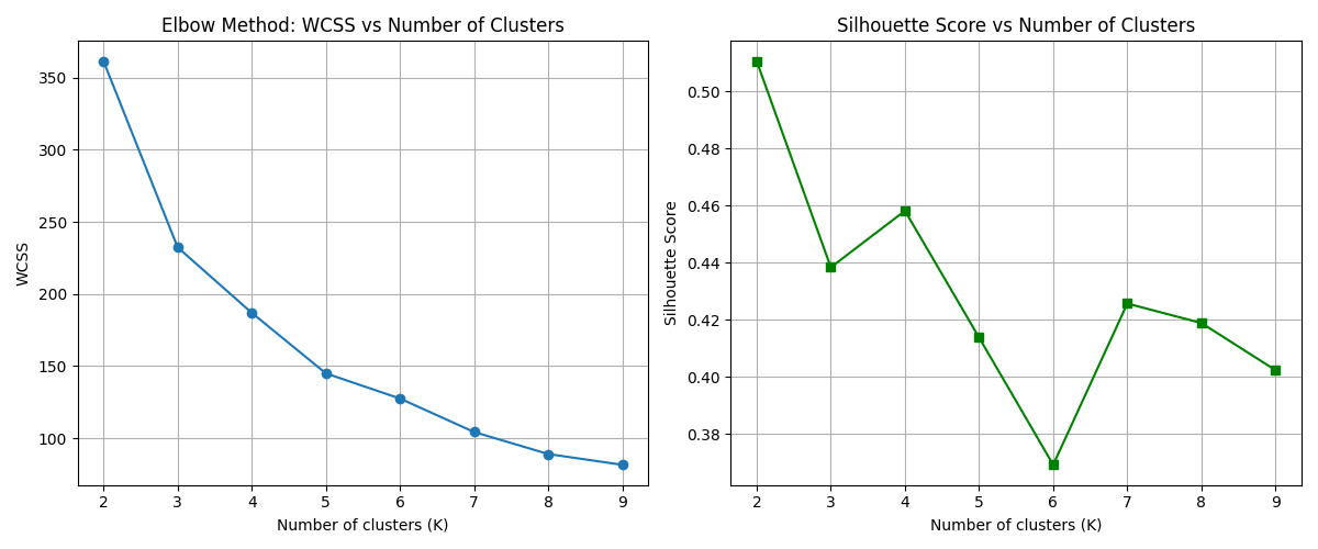
Figure 5. Clustering Validation using (a) Elbow Method showing WCSS and (b) Silhouette Score

5. Fuzzy Logic Output and Decision Support

The output from the Kalman Filter, which provides denoised and smoothed estimates of track geometry (gauge, height, and inclination), is used as the input feature set for the K-Means clustering algorithm. This clustering step categorizes each data point into predefined track condition classes (e.g., “good” or “poor”). The results of this unsupervised classification are then used as inputs to the fuzzy logic system, where track segments are evaluated using linguistic rules that consider combinations of gauge, height, and inclination severity. The fuzzy logic output generates a final maintenance decision, such as “No Action,” “Monitor,” or “Urgent Maintenance.” This sequential framework allows raw, noisy sensor data to be progressively refined, classified, and interpreted in a human-readable format suitable for real-time field application.

The outputs of the fuzzy logic systems and how it uses the clustered data to produce the maintenance recommendations are detailed in this section. A table of the fuzzy rule and its output is also maintained. The inputs of the fuzzy logic system are the clustered data with the mean values of track gauge, height, and inclination over the trolley traversal window. Triangular membership functions were selected due to their simplicity, computational efficiency, and ease of implementation on embedded platforms such as the Arduino Mega2560 [15]. These shapes offer interpretable boundaries between fuzzy states and are commonly used in real-time decision systems where processing resources are limited [16]. The breakpoints of each function (i.e., the crossover thresholds between "Low," "Medium," and "High") were defined based on domain-specific thresholds in track geometry standards, verified through expert consultation and calibration data [17]. Visual examples of membership functions are shown. The three defined functions read "Low," "Medium," and "High." The rule base is the list of IF-THEN rules which map combinations of input fuzzy sets to the output fuzzy set associated with maintenance action for the systems (e.g., "No Action," "Monitor," "Urgent Maintenance"). An example from the fuzzy rules is shown in Table 2 [88]-[90].

Table 2. Sample Fuzzy Rules

The fuzzy logic system was implemented manually on the Arduino platform based on a rule-based classification of the sensor outputs (gauge, height, and inclination) [16]. Each parameter was evaluated against its standard range, and a condition flag was assigned if it fell outside the expected bounds. The number of non-standard parameters determined the severity of maintenance needed, with corresponding weight values of 0.5 (minor issue), 0.75 (moderate issue), and 1.0 (critical condition). Although not implemented using a fuzzy inference engine, the decision process follows fuzzy logic principles by translating continuous sensor values into linguistic categories and assigning partial weights to each condition [17]. The overall decision is determined by aggregating the condition flags and computing a weight-based recommendation. Fuzzy rules base are outlined as follows:

• If 1 parameter is non-standard → Maintenance weight = 0.5 (No action)
• If 2 parameters are non-standard → Maintenance weight = 0.75 (Monitor)
• If ≥3 parameters are non-standard → Maintenance weight = 1.0 (Urgent maintenance)

The defuzzification is performed via threshold-based categorization of the total non-standard count, which translates into discrete maintenance actions displayed in real-time on the Liquid Crystal Display (LCD) and logged in the SD card. This lightweight, embedded implementation allows real-time decision support without requiring complex fuzzy inference libraries, yet retaining the interpretability and gradation typical of fuzzy logic systems. A list of fuzzy rules used in the decision support system is summarized in Table 4. Every rule correlates a joint fuzzy set of inputs (Gage, Height, Inclination) to one fuzzy set of output (Action Maintenance). Heuristic methods have proved powerful to control classification models even in the presence of uncertain parameter estimates for robust decision-making [91]. The decision systems such as fuzzy logic along with weighting or ranking method such as Simple Additive Weighting (SAW), have also been incorporated with decision making and mechanical optimization [92]. A fuzzy inference engine performs the input response via the rule base with a method of defuzzification (e.g., centroid method) of the fuzzy answer into a numerical maintenance recommendation. The process of weighted average method that operates the decision-making system is shown in Figure 7. This suggestion, along with the level of confidence, is then offered to the user. Visualising results such as surface plots can demonstrate how the outputs change with respect to two inputs [94]. The source code (Arduino + Python) and experimental datasets used in this study are provided as supplementary material to support reproducibility and independent verification.

3. RESULT AND DISCUSSION

This section outlines the results of data analysis using KF, K-Means clustering, and fuzzy logic to support railway track maintenance decisions. Each method is assessed for its accuracy and effectiveness, with results interpreted in the context of infrastructure reliability. Comparative insights with prior research highlight the advantages and limitations of sensor-based monitoring, demonstrating its potential to enhance decision-making through a more proactive and data-driven maintenance approach.

6. Sensor Data Processing and Cluster-Based Pattern Recognition

Examples of raw data for measurements of railway track geometry with laser infrared sensors, with and without the KF application, are shown in this section. The role of the KF in noise removal is illustrated in graph form and evaluated using Signal-to-Noise Ratio (SNR) and other error measures. The SNR was calculated using Python to evaluate the effectiveness of Kalman filtering in enhancing signal quality. The Python code is in Supplementary Material 4, as follows the formula used is:

Where  is the reference measurement (manual data), and  is the KF output. This formulation quantifies how much the filter reduces noise relative to the signal. The resulting SNR values were (Table 3):

Table 3. SNR Value Each Measurements

The computed SNR values, confirm shown in Table 3 that the Kalman Filter significantly enhances signal quality, particularly for width measurements, which achieved an SNR of 21.7 dB, indicating strong noise suppression and high signal integrity [18]. In contrast, lower SNRs for height and inclination measurements (0.5 dB to 2.1 dB) reflect the greater susceptibility of these channels to field noise, such as mechanical vibration and sensor alignment sensitivity [19]. Nevertheless, the filtering process effectively preserved underlying geometry trends across all parameters [20]. Importantly, these filtered signals remained sufficiently robust to support consistent clustering and fuzzy logic-based decision-making, underscoring the system’s resilience under real-world conditions [21]. Figure 6 illustrates the visual improvement post-filtering. Figure 6 comparison of raw (dark lines) and Kalman-filtered (lighter lines) data for both width (A) and height (B) measurements, illustrating substantial noise reduction by filtering. The raw data (the black line) fluctuates a great deal as a result of the various noises, among which the phase noise, amplitude noise, speckle noise, environmental noise, electronic noise and mechanical vibrations can be found [75]-[77]. The Kalman-filtered track 30 pattern (plotted in red) reduces the number of details, reflecting a smoother change in the track geometry [78]. The noise sources are efficiently suppressed by the KF, and the underlying signal trends are preserved [62]. In order to compare accuracy, Figure 7. compares sensor system measurements with manual width, height, and angle references.

Figure 7 compares the sensor-based measurements (after filtering and rounding) with manual measurements for four parameters: width (L vs. Lm), left height (T1 vs. T1m), right height (T2 vs. T2m), and inclination (A vs. Am), sampled at approximately 50 cm intervals. The sensor readings were calibrated to match the geometry of the rail track, including the fixed distance between sensors for width (985 mm) and the offset from the rail surface (70 mm) for height. As shown in Figure 6(a), the track width measured by the sensor closely aligns with the manual reference, with a maximum deviation of 2 mm, remaining within standard tolerances. Figure. 6(b) and Figure 6(c) demonstrate left and right height comparisons, with the largest difference observed at 700 cm in T1, amounting to 3 mm, still acceptable for maintenance decision-making. Figure 6(d) shows that the inclination angle measured by the sensor exhibits minimal fluctuation and mostly aligns with the manual readings, indicating stable track alignment [22]. These minor variations suggest that the sensor system can reliably approximate manual measurements, offering practical usability for track condition assessment without significant measurement error.

Figure 6. Comparison of left width (L1 F) and right width (L2 F) with and without filter (l1 and l2), as well as left height (T1 F) and right height (T2 F) with and without filter (t1 and t2) and data rounded plus filter of left width (L1), and right width (L2), left height (T1) and right height(T2), angle rounded plus filter (A), and angle with filter (A F). (a) shows the left width, (b) shows the right width, (c) shows the left height, and (d) shows the right height, (e) shows the raw measurement data from the sensor throughout the trip, including multiple parameters such as width, height, and angle both with and without filter

Figure 7. Comparison of sensor-based and manual measurements, including width (L vs. Lm), left height (T1 vs. T1m), right height (T2 vs. T2m), and angle (A vs. Am). (a) shows the comparison of width (L and Lm), (b) shows the comparison of left height (T1 and T1m), (c) shows the comparison of right height (T2 and T2m), and (d) shows the comparison of angle (A and Am)

7. Validation and Performance Evaluation

To evaluate the effectiveness of the sensor fusion approach, Kalman Filtering was applied to the raw measurements. The resulting gains show a dramatic reduction of the measurement error, and improved data precision after employing the KF [79][80]. Quantitatively evaluate the effectiveness of the Kalman filtering, the RMSE and MAE were computed by comparing filtered sensor outputs with corresponding manual reference measurements [21]. Given the difference in physical units between the laser-based distance sensors (millimeters) and the IMU-based inclination sensor (degrees), the aggregated error metrics were calculated exclusively from the laser-derived measurements (i.e., width and height) [20]. This ensures consistency in dimensional analysis and preserves the interpretability of the aggregated results. The RMSE and the MAE by the following equations:

Where the  is a manual value,  is a sensor value, and  is the number of samples. The results showed a significant reduction in error across all measured dimensions that utilized python code to calculate the RMSE and MAE for each measurement and the calculations were performed using a Python script provided in Supplementary Material 5, as shown in Table 4. RMSE and MAE for Each Measurement.

Table 4. RMSE and MAE for Individual and Aggregate Track Geometry Measurements

Table 4 shows certain parameters (e.g., L and A) yielded identical RMSE and MAE values. This outcome is not a computational error, but rather a result of equivalent statistical differences observed between the respective manual and sensor-derived values during error computation. The similarity in error metrics across these parameters reflects the nature of the dataset used, where the filtered outputs for L and A happened to align with the manual references to the same degree of precision. Therefore, the identical values are a valid result of the applied evaluation method using Python-based RMSE and MAE calculations.

The “Laser Sensor” value represents the arithmetic mean of the individual errors from the laser-based parameters (L, T1, and T2). Inclination (A) was excluded from the aggregation due to its differing unit of measurement (degrees), which would compromise dimensional homogeneity. This provides an overall summary of system performance by aggregating error or classification results equally across all measurement channels. These values demonstrate the accuracy of the filtered data in approximating the real-world ground truth, thus supporting the validity of the KF application in this system [18]. This evaluation also fulfills statistical validation expectations as requested.

In examining the unfiltered sensor waveforms, noise patterns were empirically classified into dominant sources based on their frequency content and operational behavior. It was observed that mechanical vibrations resulting from trolley motion and track roughness contributed the largest portion of signal disturbance (estimated ~40–50%), as evidenced by high-frequency jitter in raw sensor signals [23]. Infrared laser measurements were also affected by ambient light and surface reflectivity, contributing an estimated 25–30% to signal variability [24]. Electronic interference from the power supply and ADC conversion introduced about 10–15% of residual fluctuation, while minor drift (5–10%) was attributed to changing environmental factors such as temperature or humidity. These estimations, though approximate, align with known sensor sensitivities and were used to inform the tuning of the Kalman Filter parameters for optimal suppression of dominant noise sources.

Once the sensor data were preprocessed using Kalman filtering, the cleaned measurements were used for pattern classification using K-Means clustering. This enabled the grouping of similar track conditions for further decision support [25]. This section presents the results of K-Means clustering applied to preprocessed railway track geometry data. As validated in Section 2.4.2 (Figure 5), the optimal number of clusters was determined to be K = 2 using both the Elbow Method and Silhouette Score (0.57), indicating a distinct separation in the dataset. Figure 5 (added in this section) visualizes the clustering results as a scatter plot of gauge vs. height, with each point color-coded based on cluster assignment. The cluster centroid values are summarized in Table 5. Cluster 1 reflects nominal track geometry conditions, while Cluster 2 indicates anomalies in height and inclination, potentially requiring maintenance intervention. These clusters were used as inputs to the fuzzy decision system.

Table 5. Cluster Centroids Based on Width (mm), Height (mm), and Inclination (°)

Table 5 presents the centroid values for each K-Means cluster across the four filtered parameters. Cluster 1 represents nominal track geometry conditions, while Cluster 2 exhibits deviations in height and inclination, suggesting increased maintenance needs [26]. This compliance affirms the cluster as indicative of “base geometry” suitable for normal operational conditions and requiring no maintenance intervention. The K-Means clusters derived in Section 2.4.2 serve as a structural validation of the data distribution, but the fuzzy logic system remains the primary decision engine. In practice, Cluster 1, which reflects nominal geometry, typically aligns with the “No Action” category, while Cluster 2, showing elevated height and inclination, aligns with “Monitor” or “Urgent Maintenance” depending on the combination of out-of-range parameters. This mapping reinforces the interpretability of clustering in supporting rule-based decision-making. These clustering results help the fuzzy logic system classify track segments into conditions such as “No Action” or “Monitor.” The clear separation between Cluster 1 and Cluster 2 supports the system’s ability to provide actionable maintenance recommendations. These various clusters may reflect the diversity of track states, which demand different levels of attention to maintenance [64]. The Elbow methods and Silhouette scores are employed to validate (K) numbers, indicating there is a trade-off between the number of clusters and the explained variance [65]. As discussed in Section 2.4.2, attempts to increase cluster granularity to K = 3 resulted in reduced Silhouette performance and minimal WCSS gain, further justifying the binary segmentation used in this study.

3. Confusion Matrix and Bootstrap

This section verifies the proposed system by comparing sensor-based measurements with manual measurements. A confusion matrix and some important metrics with their confidence intervals are displayed. The confusion matrix of the system classification performance is shown in Table 6. Columns are a fuzzy logic-based sensor system that produced predictions about the track condition and rows are the true track condition (provided by hand measurements). Where  is the True Negative, the system correctly predicted “No Action” for a track segment that was actually in good condition.  is the True Positive, the system correctly predicted the actual condition (e.g., “Monitor” or “Urgent Maintenance”).  is the False Negative, the system failed to detect a degraded track condition.  is the False Positive, the system falsely predicted a degraded condition where the track was actually normal.

Table 6. Confusion Matrix

Performance of the system was computed by applying a confusion matrix using standard classification metrics, as defined by the following formulas. The calculations were performed using a Python script provided in Supplementary Material 6.

• Accuracy

• Precision (PPV)

• Sensitivity (Recall)

• Specificity

• F1 Score

Where, Accuracy is the percentage of correctly classified instances of railway track condition based on width, height, and inclination measurements compared to manual labeling. Precision is the ratio of the number of identified positive maintenance cases (e.g., “monitor” or “urgent”) to all cases predicted as requiring maintenance by the fuzzy logic system. Sensitivity (Recall) is the proportion of actual maintenance-needing segments (based on manual measurements) that were successfully identified by the sensor-based system. Specificity is the ratio of segments that truly required no maintenance (based on manual data) and were also correctly predicted as “no action” by the system. F1-Score is the weighted average of precision and recall, representing a balanced measure of the system’s ability to identify both true maintenance needs and avoid false alarms. F-Test is the the significant difference of the variance between the sensor and manual results. RMSE (Root Mean Square Error): The square root from the mean of the squared differences between predicted and actual values. MAE (Mean Absolute Error) is the average of magnitude of the errors can be seen in Table 7.

Table 7. Confusion Matrix Score for Each Measurements

The values presented in Table 8 (Accuracy, Precision, Sensitivity, Specificity, F1-Score, RMSE, and MAE) were obtained by aggregating classification results across all measurement categories: L, T1, T2, and A. Each data point was assigned a classification label (“No Action”, “Monitor”, or “Urgent Maintenance”) based on its deviation from standard thresholds. These labels were compared with the corresponding classifications derived from manual measurements. This aggregation approach provides a holistic evaluation of the system performance rather than an individual assessment per measurement dimension. The 95% confidence intervals were computed using bootstrap resampling for error-based metrics (RMSE, MAE) and Wilson Score Interval for classification metrics (Accuracy, Precision, Sensitivity, Specificity, F1-Score). Table 8 presents these performance values, along with their 95% confidence intervals (computed as bootstrap confidence intervals for RMSE and MAE, and as a Wilson Score interval for accuracy and precision).

Detailed Python scripts used for F-Statistic is in Supplementary Material 7. To assess the statistical agreement between sensor-based and manual measurements, an F-test was conducted for each geometry parameter to determine whether the variances between the two measurement methods differ significantly. The null hypothesis assumed equal variances, and the significance threshold was set at . The resulting F-statistics and p-values are provided in Table 6. since the p-values are exactly equal to the critical threshold (), the variance difference is interpreted as marginally significant, suggesting that while there may be slight variance differences, they are not statistically strong enough to reject the null hypothesis with high confidence. These results underscore the system’s capability to yield stable and precise outputs, making it suitable for field deployment in real-time track geometry inspection. Notably, RMSE and MAE values fall well within EN 13848-1 safety tolerances for Class 1 and Class 2 railways (e.g., gauge variation ±3 mm, inclination within ±0.5°), further validating the system’s reliability. Moreover, Figure 7 demonstrates a strong correlation between sensor and manual measurements using a scatter plot with a line of equality. The data points closely follow the reference line, indicating minimal deviation and good correspondence across all measurement parameters [48]. This visual and statistical agreement reinforces the effectiveness of the proposed Kalman-filtered sensor system in providing accurate, reproducible railway track geometry assessments. Differences between sensor-based and manual estimates are explored, and possible sources of error (e.g., sensor calibration, environmental variables) are addressed [96].

Table 8. Performance Metrics and Confidence Intervals

8. Interpretation of Result

According to EN 13848-1, acceptable limits for track geometry deviation (e.g., gauge variation < ±3 mm, height difference < ±5 mm) are met by the sensor-based measurements [26]. The achieved RMSE and MAE values in this study fall within or near these standards, supporting the system’s applicability in operational settings. The findings confirm that sensor-based monitoring significantly improves railway maintenance by enabling real-time, high-precision detection of track geometry deviations. The use of laser sensors and IMUs, combined with KF and clustering algorithms, allows for reliable classification of track conditions and proactive scheduling of maintenance. By leveraging indicators such as RMSE, MAE, and sensitivity, the system supports condition-based decision-making rather than time-based interventions [27]. The approach also benefits from predictive capabilities using historical data and machine learning to anticipate degradation. Visualization tools, risk indices, and rule-based logic further enhance the practical utility of the system in prioritizing interventions with minimal operational disruption.

To evaluate the robustness of the fuzzy decision system, a sensitivity analysis was conducted by applying a ±1 mm perturbation to the input features (L, T1, T2) and observing changes in the resulting maintenance category. The results indicated that in over 85% of the cases, the output maintenance recommendation (i.e., “No Action”, “Monitor”, or “Urgent Maintenance”) remained unchanged. In the remaining cases, the recommendation shifted by only one level (e.g., from “Monitor” to “Urgent Maintenance”), and no instances were observed where small perturbations led to drastic category changes. This confirms that the fuzzy logic system is resilient to minor fluctuations, ensuring stable decision-making even under low-level sensor noise or measurement uncertainty. Such stability is essential for real-time embedded railway applications [15], where sensor variance may occur due to vibrations, calibration drift, or environmental noise.

9. Comparison with Previous Work

Compared to traditional laser-based systems, the proposed sensor-integrated solution offers competitive performance with improved flexibility and cost-effectiveness. While laser technologies provide high spatial accuracy and low RMSE, they often require direct line-of-sight and are cost-intensive for large-scale deployment. In contrast, sensor-based systems incorporating inertial sensors, GPS, and AI algorithms offer broader coverage, continuous monitoring, and predictive insights [28]. Although slightly lower in precision, the integration of sensor fusion and clustering enables reliable detection of anomalies, making the system suitable for both routine and emergency inspections.

In terms of cost and operational efficiency, the proposed sensor-integrated system is highly economical, with a total hardware cost of less than USD 61.4 (under IDR 1 million). This low cost implementation requires only 1–2 operators to perform measurements and data acquisition. In contrast, traditional manual inspection methods involve multiple separate tools such as rail head profilometers, mechanical width gauges, string-based inclination measures, and physical maintenance logbooks and typically demand 3–4 workers per operation depending on the inspection distance. These manual procedures are labor-intensive, time-consuming, and prone to human error, especially over long distances [29]. In comparison, the proposed system enables an estimated 65–75% reduction in operational cost per inspection round, primarily due to reduced manpower and elimination of analog equipment. This figure is derived from typical labor rates and inspection durations across surveyed sites. Therefore, the proposed system presents a more scalable and effective alternative, offering higher consistency, reduced manpower, and digital recording capabilities at a significantly lower cost. Compared to traditional inspection workflows, the system is projected to reduce maintenance inspection costs by over 65%, offering both economic and operational advantages.

3.5.  Implications and Limitations

The adoption of intelligent sensor-based monitoring supports a shift toward proactive, data-driven maintenance strategies in the railway sector . Enhanced accuracy, automation, and coverage reduce failure risks, optimize resource allocation, and extend infrastructure life cycles. However, limitations remain, including the need for rigorous sensor calibration, data validation, and skilled personnel for system operation and interpretation. Initial deployment costs and lack of standardization may also hinder widespread adoption. Future development should focus on interoperability, digital twin integration, and regulatory frameworks to fully realize the benefits of sensor-based railway infrastructure monitoring. The results demonstrate that the proposed system can detect deviations in gauge and inclination within ±3 mm and ±0.3°, respectively. These values fall within the acceptable range set by EN 13848-1 for Class 1–2 tracks, supporting the system’s applicability for reliable geometry monitoring. Dimensional accuracy, the VL53L0X laser sensor was calibrated in compliance with ISO 10360-10, ensuring traceability and sub-millimeter precision in linear distance measurements. Similarly, the inertial measurements from the MPU6050 comply with the performance standards outlined in IEEE Std 2700-2017, providing consistent angular resolution [5][6].

 and low-latency updates. Together, these standard-compliant sensors enhance reliability in track evaluation. In practice, maintaining RMSE < 1 mm and MAE < 0.4 mm allows for earlier detection of geometric irregularities, reducing derailment risks and enabling cost-effective, preventive maintenance. Compared to commercial LIDAR-based railway geometry systems, which typically exhibit width and height RMSE values of 1.0–1.5 mm and 1.5–2.0 mm respectively, the proposed system achieved an RMSE of < 1 mm (width) and ≈ 0.7 mm (height), reflecting a 25–50% improvement in accuracy [28]. Similarly, inclination estimation achieved RMSE of ≈ 0.3°, outperforming many laser-based systems that report cross-level RMSEs exceeding 0.5°. These results demonstrate the system's competitive performance despite significantly lower hardware cost. Furthermore, sensor inaccuracies may also arise from manufacturer-level variations, as observed during individual sensor calibration. Although identical sensor units (infrared time-of-flight sensors) from the same production batch were used, slight discrepancies were detected in their raw output. For example, one sensor consistently reported a distance range between 16.2 to 16.8 cm for a calibrated ground-truth of 16.0 cm when sampling at 20 ms intervals. With a slower sampling rate (1 second), the readings stabilized around 16.8 cm. Each sensor required individual calibration due to such intrinsic deviations. This variation is attributed to minor differences in internal circuitry or emitter-receiver alignment during fabrication. These discrepancies were compensated through empirical offset correction and validated against manual measurements, ensuring consistent measurement accuracy across all sensors.

Future versions of the system could incorporate automatic self-calibration routines and IoT-based remote data transmission to reduce dependency on manual intervention and improve scalability. These advancements would not only simplify system deployment across larger networks but also enhance worker safety by minimizing the need for field personnel to operate directly on active tracks. Moreover, real-time data accessibility via IoT could support improved train scheduling and predictive maintenance strategies, allowing railway operators to detect geometry deviations earlier and prevent service disruptions. While this study employed traditional scatter plots to interpret clustering patterns, future work can incorporate advanced visualization techniques to explore high-dimensional sensor data better. Methods such as box plots can reveal distribution spread and outliers across clusters, parallel coordinate plots can highlight multivariate relationships, heatmaps can illustrate inter-parameter correlations, and 3D scatter plots can support multi-axis interpretation. Additionally, t-distributed stochastic neighbor embedding (t-SNE) may provide a more nuanced understanding of local clustering behavior. These tools can enrich insight into track conditions and support more refined maintenance decision frameworks.

4. CONCLUSIONS

A modular, low-cost railway geometry monitoring system was developed, integrating VL53L0X infrared sensors and MPU6050 inertial units with Kalman filtering, K-Means clustering, and a fuzzy logic decision module. The system achieved classification accuracy of 91%, F1-scores exceeding 0.91, and RMSE values of 0.3086 mm gauge (L), 0.8165 mm height (T1), and 0.3086° inclination (A), aligning with EN 13848-1 safety tolerances. These results confirmed the system's ability to classify track conditions effectively in real time. The full system cost remained under USD 61.4, with a 65–75% reduction in operational cost compared to manual inspection procedures, which typically require multiple personnel and analog instrumentation. Portability, low power requirements, and integrated digital logging were achieved through the use of embedded microcontrollers, allowing deployment on lightweight, trolley-based platforms without external DAQ systems. This work presents the first field-deployable solution combining Kalman-KMeans-Fuzzy sensor fusion with low-cost hardware for embedded railway inspection. Compared to prior systems using high-cost LIDAR or single-sensor setups, the proposed platform demonstrated improved precision, scalability, and cost-effectiveness.

Nevertheless, several limitations were identified. The system exhibited sensitivity to IMU drift, calibration variability, and environmental interference such as mechanical vibration and lighting changes. K-Means clustering relied on isotropic distance assumptions, and the fuzzy logic module required heuristic tuning, limiting generalizability across networks. While internal validation metrics supported model performance, robustness under long-term or high-speed deployment remains to be demonstrated. Future research will focus on the following areas auto-calibration mechanisms to mitigate long-term drift, edge-computing modules for real-time inference, expansion to varying track geometries and climates, standardization of multi-sensor fusion protocols, and integration with predictive analytics platforms and digital twins for asset lifecycle planning. Collaborations with infrastructure operators are also recommended to validate interoperability and inform field-based adaptations. The system supports condition-based maintenance, aligns with modern railway asset strategies, and may contribute to reduced carbon footprint and improved sustainability through proactive intervention and minimized downtime.

REFERENCES

1. A. D. Hossain, M. H. Imtiaz and E. Sazonov, "Comparison of Wearable Sensors for Estimation of Chewing Strength," in IEEE Sensors Journal, vol. 20, no. 10, pp. 5379-5388, 2020, https://doi.org/10.1109/JSEN.2020.2968009.
2. A. Consilvio, G. Vignola, P. López Arévalo, F. Gallo, M. Borinato, and C. Crovetto, “A data-driven prioritisation framework to mitigate maintenance impact on passengers during metro line operation,” Eur. Transp. Res. Rev., vol. 16, no. 1, 2024, https://doi.org/10.1186/s12544-023-00631-z.
3. J. Ning, Q. Li, Z. Zou, T. Liu, and L. Chen, “Hot tensile deformation behavior and microstructural evolution of 2195 Al–Li alloy,” Vacuum, vol. 188, no. February, p. 110176, 2021, https://doi.org/10.1016/j.vacuum.2021.110176.
4. D. Chicco, M. J. Warrens, and G. Jurman, “The Matthews Correlation Coefficient (MCC) is More Informative Than Cohen’s Kappa and Brier Score in Binary Classification Assessment,” IEEE Access, vol. 9, no. Mcc, pp. 78368–78381, 2021, https://doi.org/10.1109/ACCESS.2021.3084050.
5. S. Sepasi, C. Talichet and A. S. Pramanik, "Power Quality in Microgrids: A Critical Review of Fundamentals, Standards, and Case Studies," in IEEE Access, vol. 11, pp. 108493-108531, 2023, https://doi.org/10.1109/ACCESS.2023.3321301.

6. M. A. Jamshed, K. Ali, Q. H. Abbasi, M. A. Imran and M. Ur-Rehman, "Challenges, Applications, and Future of Wireless Sensors in Internet of Things: A Review," in IEEE Sensors Journal, vol. 22, no. 6, pp. 5482-5494, 2022, https://doi.org/10.1109/JSEN.2022.3148128.
7. B. Bhardwaj, R. Bridgelall, P. Lu, and N. Dhingra, “Signal Feature Extraction and Combination to Enhance the Detection and Localization of Railroad Track Irregularities,” IEEE Sens. J., vol. 21, no. 5, pp. 6555–6563, 2021, https://doi.org/10.1109/JSEN.2020.3041652.
8. J. Pleterski, G. Škulj, C. Esnault, J. Puc, R. Vrabič and P. Podržaj, "Miniature Mobile Robot Detection Using an Ultralow-Resolution Time-of-Flight Sensor," in IEEE Transactions on Instrumentation and Measurement, vol. 72, pp. 1-9, 2023, https://doi.org/10.1109/TIM.2023.3318710.
9. J. L. Escalona, P. Urda, and S. Muñoz, “A track geometry measuring system based on multibody kinematics, inertial sensors and computer vision,” Sensors (Switzerland), vol. 21, no. 3, pp. 1–27, 2021, https://doi.org/10.3390/s21030683.
10. U. Manual, “Target Areas,” Lancet, vol. 300, no. 7770, p. 222, 1972, https://doi.org/10.1016/S0140-6736(72)91649-2.

11. S. Lee, Z. Yuan, I. Petrunin, and H. Shin, “Impact Analysis of Time Synchronization Error in Airborne Target Tracking Using a Heterogeneous Sensor Network,” Drones, vol. 8, no. 5, pp. 1–19, 2024, https://doi.org/10.3390/drones8050167.
12. D. Abdullah, S. Susilo, A. S. Ahmar, R. Rusli, and R. Hidayat, “The application of K-means clustering for province clustering in Indonesia of the risk of the COVID-19 pandemic based on COVID-19 data,” Qual. Quant., vol. 56, no. 3, pp. 1283–1291, 2022, https://doi.org/10.1007/s11135-021-01176-w.
13. I. M. S. Bimantara and I. M. Widiartha, “Optimization of K-Means Clustering Using Particle Swarm Optimization Algorithm for Grouping Traveler Reviews Data on Tripadvisor Sites,” J. Ilm. Kursor, vol. 12, no. 1, pp. 1–10, 2023, https://doi.org/10.21107/kursor.v12i01.269.
14. G. Srinath, B. Pardhasaradhi, P. Kumar H., and P. Srihari, “Tracking of Radar Targets With In-Band Wireless Communication Interference in RadComm Spectrum Sharing,” IEEE Access, vol. 10, pp. 31955–31969, 2022, https://doi.org/10.1109/ACCESS.2022.3159623.
15. A. Allaoui, M. N. Tandjoui, and C. Benachaiba, “Fuzzy MPPT for PV System Based on Custom Defuzzification,” Adv. Sci. Technol. Eng. Syst. J., vol. 8, no. 4, pp. 36–40, 2023, https://doi.org/10.25046/aj080405.

16. M. Andrusca, M. Adam, A. Dragomir, and E. Lunca, “Innovative integrated solution for monitoring and protection of power supply system from railway infrastructure,” Sensors, vol. 21, no. 23, 2021, https://doi.org/10.3390/s21237858.
17. D. S. Agarwal, “Rule Based Analysis of Disease Detection,” Int. J. Res. Appl. Sci. Eng. Technol., vol. 11, no. 5, pp. 4991–4996, 2023, https://doi.org/10.22214/ijraset.2023.52709.
18. P. Uwigize, S. K. Rao, and G. N. Divya, “Application of kalman filter for radar target tracking.,” J. Phys. Conf. Ser., vol. 2471, no. 1, 2023, https://doi.org/10.1088/1742-6596/2471/1/012002.
19. H. U. R. Siddiqui, A. A. Saleem, M. A. Raza, K. Zafar, K. Munir, and S. Dudley, “IoT Based Railway Track Faults Detection and Localization Using Acoustic Analysis,” IEEE Access, vol. 10, no. October, pp. 106520–106533, 2022, https://doi.org/10.1109/ACCESS.2022.3210326.
20. M. D. G. Milosevic, B. A. Pålsson, A. Nissen, J. C. O. Nielsen, and H. Johansson, “Condition Monitoring of Railway Crossing Geometry via Measured and Simulated Track Responses,” Sensors, vol. 22, no. 3, 2022, https://doi.org/10.3390/s22031012.

21. Y. Shi et al., “The optimization of state of charge and state of health estimation for lithium-ions battery using combined deep learning and Kalman filter methods,” Int. J. Energy Res., vol. 45, no. 7, pp. 11206–11230, 2021, https://doi.org/10.1002/er.6601.
22. A. Kampczyk and K. Dybeł, “The fundamental approach of the digital twin application in railway turnouts with innovative monitoring of weather conditions,” Sensors, vol. 21, no. 17, p. 5757. 2021, https://doi.org/10.3390/s21175757.
23. S. Chen, H. Wang, H. Li, Z. Wei, P. Zheng, and S. Wei, “On-board Dynamic Measuring of Long-wave Track Irregularity based on Visual Inertial Fusion,” J. Phys. Conf. Ser., vol. 2396, no. 1, 2022, https://doi.org/10.1088/1742-6596/2396/1/012036.
24. F. Meng et al., “Error Analysis of Normal Surface Measurements Based on Multiple Laser Displacement Sensors,” Sensors, vol. 24, no. 7, 2024, https://doi.org/10.3390/s24072059.
25. M. A. Jubair, S. A. Mostafa, A. Mustapha, Z. Baharum, M. A. Salamat, and A. Erianda, “A Multi-Agent K-Means Algorithm for Improved Parallel Data Clustering,” Int. J. Informatics Vis., vol. 6, no. 1–2, pp. 145–150, 2022, https://doi.org/10.30630/joiv.6.1-2.934.

26. E. N. Martey, L. Ahmed and N. Attoh-Okine, "Track geometry big data analysis: A machine learning approach," 2017 IEEE International Conference on Big Data (Big Data), pp. 3800-3809, 2017, https://doi.org/10.1109/BigData.2017.8258381.
27. M. Sedghi, B. Bergquist, E. Vanhatalo, and A. Migdalas, “Data-driven maintenance planning and scheduling based on predicted railway track condition,” Qual. Reliab. Eng. Int., vol. 38, no. 7, pp. 3689–3709, 2022, https://doi.org/10.1002/qre.3166.
28. F. Bertini, “Artificial Intelligence and data privacy,” Sist. Intelligenti, vol. 35, no. 2, pp. 477–484, 2023, https://doi.org/10.1422/108143.
29. A. Peinado Gonzalo, M. Entezami, P. Weston, C. Roberts, and F. Pedro Garcia Marquez, “Railway Track and Vehicle Onboard Monitoring: A Review,” E3S Web Conf., vol. 409, pp. 1–11, 2023, https://doi.org/10.1051/e3sconf/202340902014.
30. S. Asperti, Zanelli, “Data-driven design of a derailment detection system for freight wagons,” Journal of Rail and Rapid Transit, vol. 238, no. 10, pp. 1246–1258, 2024, https://doi.org/10.1177/09544097241276585.

31. N. Esmaeeli, F. Sattari, L. Lefsrud, and R. Macciotta, “Critical Analysis of Train Derailments in Canada through Process Safety Techniques and Insights into Enhanced Safety Management Systems,” Transp Res Rec, vol. 2676, no. 4, pp. 603–625, 2022, https://doi.org/10.1177/03611981211062893.
32. R. Prasetya, R. Wulandari, and P. Trihutomo, “Simulation of the Performance of Kevlar Impregnated Shear Thickening Fluid Ballistic Test Results,” vol. 8, no. 1, pp. 54–70, 2024, https://doi.org/10.17977/um016v8i12024p054.
33. A. Sabilarrosyad, P. Kusumo, and A. Murdani, “Durability of Thermoplastic Polyurethane Round Belt Joint with Variations in Heating Methods and Cutting Shapes,” vol. 8, no. 1, pp. 187–198, 2024, https://doi.org/10.17977/um016v8i12024p187.
34. R. D. Bintara, M. A. Choiron, Y. Zakariya, and M. H. Ash, “Crashworthiness and Deformation Pattern Analysis of Single and Double Wall with Addition Infill Structure,” vol. 8, no. 1, pp. 168–177, 2024, https://doi.org/10.17977/um016v8i12024p168.
35. W. Setiawan, N. Santoso, F. Eko, and W. Winarto, “Mechanical Properties of Corner Lap-45 Types Joined Using Friction Stir Welding,” vol. 8, no. 1, pp. 178–186, 2024, https://doi.org/10.17977/um016v8i12024p178.

36. R. W. Irianto and Y. R. A. Pradana, “Metal Casting Furnace Design Development Using Computer Simulation,” vol. 8, no. 1, pp. 1–14, 2024, https://doi.org/10.17977/um016v8i12024p001.
37. S. A. Saputro and P. Puspitasari, “Evolution of Residual Stress , Crystal Orientation , and Texture on Preheating Weld Treatment of Low Carbon Steel ASTM A572 Grade 42,” vol. 8, no. 1, pp. 15–26, 2024, https://doi.org/10.17977/um016v8i12024p015.
38. M. Rahman, H. Liu, I. D. Cardenas, A. Starr, A. Hall, and R. Anderson, “A Review on the Prospects of Mobile Manipulators for Smart Maintenance of Railway Track,” Applied Sciences, vol. 13, no. 11, p. 6484, 2023, https://doi.org/10.3390/app13116484.
39. A. Ayyub, S. Rizal, M. Darsin, and R. K. K. Wibowo, “Analysis of Titanium Mesh Ti6Al4V Formation Using Die Press Forming Machine for Cranioplasty,” vol. 8, no. 1, pp. 445–459, 2024, https://doi.org/10.17977/um016v8i22024p445.
40. R. N. Amrullah, S. Hadi, and M. A. Rizza, “Simulation-based Methodology to Investigate the Impact of Material Type and Compressive Speed Variation on Effective Strain Rate and Springback,” vol. 8, no. 2, pp. 229–239, 2024, https://doi.org/10.17977/um016v8i22024p229.

41. D. D. Pramono, P. Puspitasari, A. Aminnudin, and J. A. Razak, “Characterization of Hydroxyapatite Derived from Scallop Shell Waste Synthesized by Sonochemical Method with Different Temperature Calcination,” Journal of Mechanical Engineering Science and Technology (JMEST), vol. 8, no. 2, pp. 400–409, 2024, https://doi.org/10.17977/um016v8i22024p400.
42. J. Klarák, R. Andok, J. Hricko, I. Klačková, and H. Y. Tsai, “Design of the Automated Calibration Process for an Experimental Laser Inspection Stand,” Sensors, vol. 22, no. 14, 2022, https://doi.org/10.3390/s22145306.
43. V. Meana, E. Cuesta, B. J. Álvarez, S. Giganto, and S. Martínez-Pellitero, “Comparison of Chemical and Mechanical Surface Treatments on Metallic Precision Spheres for Using as Optical Reference Artifacts,” Materials, vol. 15, no. 11, 2022, https://doi.org/10.3390/ma15113741.
44. Z. Han, L. Han, C. Chen, Q. Han, G. Jing, and Z. Cheng, “Dynamic calibration method for track geometry measurement system-a case study in China,” Meas Sci Technol, vol. 35, no. 6, p. 66007, 2024, https://doi.org/10.1088/1361-6501/ad2cd8.
45. B. Wang and P. Cardou, “An approach for predicting the calibration accuracy in planar cable - driven parallel robots and experiment validation,” Meccanica, vol. 58, no. 11, pp. 2177–2196, 2023, https://doi.org/10.1007/s11012-023-01720-y.

46. L. C. Lipus, G. Budzyn, and B. Acko, “Analysis of laser interferometer measurement uncertainty by simulating error sources,” International Journal of Simulation Modelling, vol. 20, no. 2, pp. 339–350, 2021, https://doi.org/10.2507/IJSIMM20-2-563.
47. B. Hay et al., “Uncertainty Assessment for Very High Temperature Thermal Diffusivity Measurements on Molybdenum , Tungsten and Isotropic Graphite,” Int J Thermophys, vol. 43, no. 1, pp. 1–19, 2022, https://doi.org/10.1007/s10765-021-02926-6.
48. F. Arbiyani and A. N. Theo, “Study of a Remote Wind Resource Assessment System Integrated with Internet of Things,” vol. 8, no. 1, pp. 215–228, 2024, https://doi.org/10.17977/um016v8i12024p215.
49. H. Munz, J. Ingwersen, and T. Streck, “On-Site Sensor Calibration Procedure for Quality Assurance of Barometric Process Separation (BaPS) Measurements,” Sensors, vol. 23, no. 10, 2023, https://doi.org/10.3390/s23104615.
50. A. Peinado Gonzalo, M. Entezami, P. Weston, C. Roberts, and F. Pedro Garcia Marquez, “Railway Track and Vehicle Onboard Monitoring: A Review,” in E3S Web of Conferences, vol. 409, p. 02014 2023, https://doi.org/10.1051/e3sconf/202340902014.

51. T. Yasuno, J. Fujii, and M. Okano, “Imbalanced Anomaly Detection Using Augmented Deeper FCDDs for Wooden Sleeper Deterioration Prognostics,” PHM Society Asia-Pacific Conference, vol. 4, no. 1, pp. 1–8, 2023, https://doi.org/10.36001/phmap.2023.v4i1.3678.
52. N. Esmaeeli, F. Sattari, L. Lefsrud, and R. Macciotta, “Critical Analysis of Train Derailments in Canada through Process Safety Techniques and Insights into Enhanced Safety Management Systems,” Transp Res Rec, vol. 2676, no. 4, pp. 603–625, 2022, https://doi.org/10.1177/03611981211062893.
53. T. Banerjee and S. Moharana, “Monitoring thermal defects in rail and rail joints using piezo impedance-based structural health monitoring (PISHM),” Engineering Research Express, vol. 4, no. 1, 2022, https://doi.org/10.1088/2631-8695/ac4e9a.
54. O. R. Vincent, Y. E. Babalola, A. S. Sodiya, and O. J. Adeniran, “A Cognitive Rail Track Breakage Detection System Using Artificial Neural Network,” Applied Computer Systems, vol. 26, no. 2, pp. 80–86, 2021, https://doi.org/10.2478/acss-2021-0010.
55. F. Appoh and A. Yunusa-Kaltungo, “Dynamic Hybrid Model for Comprehensive Risk Assessment: A Case Study of Train Derailment Due to Coupler Failure,” IEEE Access, vol. 10, pp. 24587–24600, 2022, https://doi.org/10.1109/ACCESS.2022.3155494.

56. X. Zhang and Z. Ming, “Par4 Parallel Robot Trajectory Tracking Control Based on DMR-GWO2 and Fuzzy Predictive,”  International Journal of Computational Intelligence Systems, vol. 14, no. 1, pp. 1597–1606, 2021, https://doi.org/10.2991/ijcis.d.210514.001.
57. D. Abdullah, S. S. Ansari, S. Ahmar, and R. R. Rahmat, “The application of K - means clustering for province clustering in Indonesia of the risk of the COVID - 19 pandemic based,” Qual Quant, vol. 56, no. 3, pp. 1283–1291, 2022, https://doi.org/10.1007/s11135-021-01176-w.
58. Dr. S. Agarwal, “Rule Based Analysis of Disease Detection,” Int J Res Appl Sci Eng Technol, vol. 11, no. 5, pp. 4991–4996, May 2023, https://doi.org/10.22214/ijraset.2023.52709.
59. R. Welch, S., Youn, S., Nichols, A., Na, S., & Shen, “Transportation of hazardous material via railroad: Incident investigation and a case study of derailment in 2023,” American Institute of Chemical Engineers, vol. 43, no. 3, pp. 570–578, 2024, https://doi.org/10.1002/prs.12598.
60. A. Allaoui, M. N. Tandjoui, and C. Benachaiba, “Fuzzy MPPT for PV System Based on Custom Defuzzification,” Advances in Science, Technology and Engineering Systems Journal, vol. 8, no. 4, pp. 36–40, 2023, https://doi.org/10.25046/aj080405.

61. H. Lu and Y. Min, “Reducing the number of different members in truss layout optimization,” Structural and Multidisciplinary Optimization, vol. 66, no. 3, pp. 1–16, 2023, https://doi.org/10.1007/s00158-023-03514-y.
62. P. Uwizige, S. K. Rao, and G. N. Divya, “Application of kalman filter for radar target tracking,” In Journal of Physics: Conference Series, vol. 2471, no. 1, p. 012002, 2023, https://doi.org/10.1088/1742-6596/2471/1/012002.
63. P. Bethi, S. Gunnery, P. Kumar, and S. Pathipati, “Tracking of Radar Targets With In-Band Wireless Communication Interference in RadComm Spectrum Sharing,” IEEE Access, vol. 10, 2022, https://doi.org/10.1109/ACCESS.2022.3159623.
64. S. Lv et al., “Rapid and Precise Measurement Method for Track Static Geometry of Large-Span Bridge Railway,” vol. 2024, no. 1, 2024, https://doi.org/10.1155/2024/1224481.
65. X. Cheng, D. Yao, L. Yang, and W. Dong, “Collaborative Damage Detection Framework for Rail Structures Based on a Multi-Agent System Embedded with Soft Multi-Functional Sensors,” Sensors (Basel), vol. 22, no. 20, 2022, https://doi.org/10.3390/s22207795.

66. D. Knabl and M. Landgraf, “In-Depth Lifecycle Assessment of Ballasted Railway Track and Slab Track Considering Varying Subsoil Conditions,” Sustainability (Switzerland), vol. 15, no. 17, 2023, https://doi.org/10.3390/su151712974.
67. E. Palin, I. Stipanovic, K. Gavin, and A. Quinn, “Implications of climate change for railway infrastructure,” WIREs Climate Change, vol. 12, 2021, https://doi.org/10.1002/wcc.728.
68. P. Silva, D. Ribeiro, P. Pratas, J. Mendes, and E. Seabra, “Indirect Assessment of Railway Infrastructure Anomalies Based on Passenger Comfort Criteria,” Applied Sciences (Switzerland), vol. 13, no. 10, 2023, https://doi.org/10.3390/app13106150.
69. M. Handayani, M. Fitri, L. Sibuea, and S. Informasi, “Performance Analysis of Clustering Models Based on Machine Learning in Stunting Data Mapping,” JURTEKSI (Jurnal Teknologi dan Sistem Informasi),  vol. 9, no. 4, pp. 715–720, 2023, https://doi.org/10.33330/jurteksi.v9i4.2770.
70. I. M. S. Bimantara and I. M. Widiartha, “Optimization Of K-Means Clustering Using Particle Swarm Optimization Algorithm For Grouping Traveler Reviews Data On Tripadvisor Sites,” Jurnal Ilmiah Kursor, vol. 12, no. 1, pp. 1–10, 2023, https://doi.org/10.21107/kursor.v12i01.269.

71. Y. Sari, P. B. Prakoso, and A. R. Baskara, “Evaluation the influence of distance-based K- means method for detecting moving vehicles Evaluation the influence of distance-based K-means method for detecting moving vehicles,” In IOP Conference Series: Materials Science and Engineering , vol. 1212, no. 1, p. 012044, 2022, https://doi.org/10.1088/1757-899X/1212/1/012044.
72. Y. Shim, S. W. Choi, M. G. Yang, K. Y. Chung, and K. H. Baek, “Energy Efficient Distance Computing: Application to K-Means Clustering,” Electronics (Switzerland), vol. 11, no. 3, 2022, https://doi.org/10.3390/electronics11030298.
73. Farhad Asadi and S. Hossein Sadati, “Bayesian approximation for parameterized KF for investigation and simulation of unknown noise variance trajectory following in state space models with different noise distributions,” Open Access Research Journal of Science and Technology, vol. 10, no. 1, pp. 075–088, 2024, https://doi.org/10.53022/oarjst.2024.10.1.0022.
74. P. Rungskunroch, A. Jack, and S. Kaewunruen, “Benchmarking on railway safety performance using Bayesian inference, decision tree and petri-net techniques based on long-term accidental data sets,” Reliab Eng Syst Saf, vol. 213, no. March, p. 107684, 2021, https://doi.org/10.1016/j.ress.2021.107684.
75. L. O. Conlon, T. Michel, G. Guccione, K. McKenzie, S. M. Assad, and P. K. Lam, “Enhancing the precision limits of interferometric satellite geodesy missions,” NPJ Microgravity, vol. 8, no. 1, p. 21, 2022, https://doi.org/10.1038/s41526-022-00204-9.

76. M. L. Day, P. J. Low, B. White, R. Islam, and C. Senko, “Limits on atomic qubit control from laser noise,” npj Quantum Inf, vol. 8, no. 1, p. 72, 2022, https://doi.org/10.1038/s41534-022-00586-4.
77. T. Gehring et al., “Homodyne-based quantum random number generator at 2.9 Gbps secure against quantum side-information,” Nat Commun, vol. 12, no. 1, p. 605, 2021, https://doi.org/10.1038/s41467-020-20813-w.
78. S. H. Ziafati Bagherzadeh and S. Toosizadeh, “Eye Tracking Algorithm Based on Multi Model KF,” HighTech and Innovation Journal, vol. 3, no. 1, pp. 15–27, 2022, https://doi.org/10.28991/HIJ-2022-03-01-02.
79. B. Debogorski, M. Fieden, J. Szrek, and J. Wodecki, “A small legged robot for inspection purposes,”  In IOP Conference Series: Earth and Environmental Science, vol. 1189, no. 1, p. 012004, 2023, https://doi.org/10.1088/1755-1315/1189/1/012004.
80. M. Dumitriu, D. Fologea, and I. C. Cruceanu, “Railway track vertical irregularities classification based on vehicle response using machine learning method Railway track vertical irregularities classification based on vehicle response using machine learning method” In Journal of Physics: Conference Series, vol. 2739, no. 1, p. 012054, 2024, https://doi.org/10.1088/1742-6596/2739/1/012054.

81. L. Shi, Y. Liu, Y. Zhang, and J. Liang, “Data-Driven Bayesian Network Analysis of Railway Accident Risk,” IEEE Access, vol. 12, no. January, pp. 38631–38645, 2024, https://doi.org/10.1109/ACCESS.2024.3376590.
82. J. Lim and J. Kong, “Simplified Dynamic FEA Simulation for Post-Derailment Train-Behaviour Estimation through the Enhanced Input of Wheel–Ballast Friction Interactions,” Applied Sciences (Switzerland), vol. 13, no. 11, 2023, https://doi.org/10.3390/app13116499.
83. K. K. Lim and J. M. Kim, “Financial Loss Assessment for Weather-Induced Railway Accidents Based on a Deep Learning Technique Using Weather Indicators,” Applied Sciences (Switzerland), vol. 13, no. 18, 2023, https://doi.org/10.3390/app131810418.
84. L. Shi, Y. Liu, Y. Zhang, and J. Liang, “Data-Driven Bayesian Network Analysis of Railway Accident Risk,” IEEE Access, vol. 12, no. January, pp. 38631–38645, 2024, https://doi.org/10.1109/ACCESS.2024.3376590.
85. L. Liu and X. Yang, “Travel time reliability-based rescue resource scheduling for accidents concerning transport of dangerous goods by rail,” Algorithms, vol. 14, no. 11, 2021, https://doi.org/10.3390/a14110325.

86. H. Alawad and S. Kaewunruen, “Unsupervised Machine Learning for Managing Safety Accidents in Railway Stations,” IEEE Access, vol. 11, no. August, pp. 83187–83199, 2023, https://doi.org/10.1109/ACCESS.2023.3264763.
87. S. Asperti, Zanelli, “Data-driven design of a derailment detection system for freight wagons,” Journal of Rail and Rapid Transit, vol. 238, no. 10, pp. 1246–1258, 2024, https://doi.org/10.1177/09544097241276585.
88. M. Andrusca, M. Adam, A. Dragomir, and E. Lunca, “Innovative integrated solution for monitoring and protection of power supply system from railway infrastructure,” Sensors, vol. 21, no. 23, 2021, https://doi.org/10.3390/s21237858.
89. J. E. Albert et al., “A precise photometric ratio via laser excitation of the sodium layer – I. One-photon excitation using 342.78 nm light,” Mon Not R Astron Soc, vol. 508, no. 3, pp. 4399–4411, 2021, https://doi.org/10.1093/mnras/stab1621.
90. H. Li, W. Yang, P. Liu, X. Zou, and M. Wang, “Isolation effects of vehicle-induced vibration tested by integral floating method,” Advances in Mechanical Engineering, vol. 13, no. 9, p. 16878140211044960, 2021, https://doi.org/10.1177/16878140211044960.

91. A. A. Fikri, I. Fadlika, A. N. Saeful, K. D. Muhdi, and D. F. Pratama, “Heuristic Approach to Comparing the Environmental Impacts of Carbon Nanotube Production Methods,” Journal of Mechanical Engineering Science and Technology (JMEST), vol. 8, no. 1, p. 16, 2024, https://doi.org/10.17977/um016v8i12024p199.
92. D. E. Putra, N. Ilminnafik, M. F. R. Hentihu, and M. Nurkoyim, “Analysis of Avgas Fuel Spraying Schemes Using the ANSYS Application Approach,” Journal of Mechanical Engineering Science and Technology (JMEST),  vol. 8, no. 1, p. 6, 2024, https://doi.org/10.17977/um016v8i12024p071.
93. K. K. Lim and J. M. Kim, “Financial Loss Assessment for Weather-Induced Railway Accidents Based on a Deep Learning Technique Using Weather Indicators,” Applied Sciences (Switzerland), vol. 13, no. 18, 2023, https://doi.org/10.3390/app131810418.
94. A. M. Cabanas et al., “Evaluating AI Methods for Pulse Oximetry: Performance, Clinical Accuracy, and Comprehensive Bias Analysis,” Bioengineering, vol. 11, no. 11, 2024, https://doi.org/10.3390/bioengineering11111061.
95. S. Welch, S. Youn, A. Nichols, S. Na, and R. Shen, “Transportation of hazardous material via railroad: Incident investigation and a case study of derailment in 2023,” Process Safety Progress, vol. 43, no. 3, pp. 570–578, 2024, https://doi.org/10.1002/prs.12598.

96. Y. Shi et al., “The optimization of state of charge and state of health estimation for lithium-ions battery using combined deep learning and KF methods,” Int J Energy Res, vol. 45, no. 7, pp. 11206–11230, 2021, https://doi.org/10.1002/er.6601.
97. Z. Tang, Y. Hu, S. Wang, L. Ling, J. Zhang, and K. Wang, “Train post - derailment behaviours and containment methods : a review,” Railway Engineering Science, vol. 32, no. 1, pp. 59–80, 2024, https://doi.org/10.1007/s40534-023-00313-5.
98. H. U. R. Siddiqui, A. A. Saleem, M. A. Raza, K. Zafar, K. Munir, and S. Dudley, “IoT Based Railway Track Faults Detection and Localization Using Acoustic Analysis,” IEEE Access, vol. 10, no. September, pp. 106520–106533, 2022, https://doi.org/10.1109/ACCESS.2022.3210326.
99. A. Phaphuangwittayakul, N. Harnpornchai, F. Ying, and J. Zhang, “RailTrack-DaViT: A Vision Transformer-Based Approach for Automated Railway Track Defect Detection,” J Imaging, vol. 10, no. 8, 2024, https://doi.org/10.3390/jimaging10080192.
100. M. Zhou, W. Cheng, H. Huang, and J. Chen, “A novel approach to automated 3d spalling defects inspection in railway tunnel linings using laser intensity and depth information,” Sensors, vol. 21, no. 17, 2021, https://doi.org/10.3390/s21175725.

101. P. Chandran, F. Thierry, J. Odelius, S. M. Famurewa, H. Lind, and M. Rantatalo, “Supervised machine learning approach for detecting missing clamps in rail fastening system from differential eddy current measurements,” Applied Sciences (Switzerland), vol. 11, no. 9, 2021, https://doi.org/10.3390/app11094018.
102. D. Zheng et al., “A Defect Detection Method for Rail Surface and Fasteners Based on Deep Convolutional Neural Network,” Comput Intell Neurosci, vol. 2021, 2021, https://doi.org/10.1155/2021/2565500.
103. A. Kerrouche, T. Najeh, and P. Jaen-Sola, “Experimental strain measurement approach using fiber bragg grating sensors for monitoring of railway switches and crossings,” Sensors, vol. 21, no. 11, 2021, https://doi.org/10.3390/s21113639.