ISSN: 2685-9572 Buletin Ilmiah Sarjana Teknik Elektro
Vol. 7, No. 4, December 2025, pp. 918-930
Effective Analysis of Machine Learning Algorithms for Breast Cancer Prediction
Vanitha M 1, V Anitha 1, Beulah Jackson 2, Anne Jenefer F 3
1 Department of Electronics and Communication Engineering, Saveetha Engineering College, Chennai, Tamilnadu, India
2 Department of Electronics and Communication Engineering, Vel Tech Rangarajan Dr. Sagunthala R&D Institute of Science and Technology, Chennai, Tamilnadu, India
3 Department of Electronics and Communication Engineering, Panimalar Engineering College, Chennai,
Tamilnadu, India
ARTICLE INFORMATION |
| ABSTRACT |
Article History: Received 16 June 2025 Revised 18 July 2025 Accepted 02 December 2025 |
| 
Early prognosis of Breast Cancer (BC) is significantly important to cure the disease easily so it is essential to develop methods that is able to aid doctors to get precise prognosis. Hence, a BC prognosis methodology is proposed utilizing Machine Learning (ML) approaches. The target of this paper is to utilize classification techniques to classify tumor types, or benign and malignant cells, using 569 samples from Wisconsin Diagnostic Breast Cancer (WDBC) database. Initially, preprocessing is employed to enhance the data’s quality, which includes data cleaning and min-max normalization. It improves the input breast cancer data's quality, accuracy, and suitability for further analysis. Followed by preprocessing, the ML approaches such as K-Nearest Neighbour (KNN), Random Forest (RF) and Support Vector Machine (SVM) methods are analyzed for the classification of BC data. Each algorithm offers a distinct approach to classification by capturing local patterns in data and handles high-dimensional spaces along with nonlinear boundaries through kernel tricks. The developed work is implemented in python software and comparative analysis is done with traditional methods. The outcomes demonstrates that the proposed KNN classifier shows better performance interms of precision, recall, F1-score with an accuracy of 96.49%, ensuring the earliest diagnosis of breast cancer compared with SVM and RF. This comparative approach enhances the reliability of the proposed methodology and supports the selection of the best-performing algorithm offering valuable insights for real-world clinical decision support systems. |
Keywords: Breast Cancer; Diagnosis; Data Preprocessing; Classification; SVM; RF; KNN |
Corresponding Author: Vanitha M, Department of Electronics and Communication Engineering, Saveetha Engineering College, Chennai, Tamilnadu, India. Email: vanitha@saveetha.ac.in |
This work is open access under a Creative Commons Attribution-Share Alike 4.0 
|
Document Citation: V. M, V Anitha, B. Jackson, and A. J. F, “Effective Analysis of Machine Learning Algorithms for Breast Cancer Prediction,” Buletin Ilmiah Sarjana Teknik Elektro, vol. 7, no. 4, pp. 918-930, 2025, DOI: 10.12928/biste.v7i4.13663. |
INTRODUCTION
Breast Cancer is one of the leading causes of cancer-related deaths globally and it arises from an irregular and accelerated development of breast cells, or tumors [1]. It is the primary reason of cancer-related mortality among women, accounting for 2.1 million cases annually [2]. The majority of these tumors fall into 2 kinds: non-cancerous or “benign”, and cancerous or “malignant” [3]. Benign tumors have clear borders and develop slowly; they never invade neighboring tissue or other body components [4]. However, cancerous tumors multiply, have uniform margins, and spread swiftly through a process known as metastasis to other bodily organs [5]. This rapid and invasive spread significantly increases the complexity of cancer treatment and lowers the likelihood of successful outcomes, especially if not detected early [6]. In addition, there are 2 types of BC: invasive cancer and ductal carcinoma in situ, which is sometimes referred to as non-invasive BC [7]. To distinguish between these malignancies, medical professionals require a dependable diagnostic method [8]. Even for specialists, it is typically difficult to detect the malignancies [9]. Manual diagnosis of breast cancer, typically performed through visual examination of imaging results and histopathological analysis, is often limited by human error, subjectivity and variability in expertise among medical professionals [10]. Factors such as fatigue, inconsistent interpretation of visual patterns and differences in diagnostic experience can lead to misclassification or delayed diagnosis, potentially affecting patient outcomes [11]. Additionally, manual processes can be time-consuming and less scalable, especially in regions with limited access to skilled pathologists [12]. These challenges highlight the need for automated, data-driven approaches using ML, which can offer consistent, objective and rapid analysis of complex data [13], thereby supporting clinicians in making more accurate and timely decisions [14]. Therefore, identifying tumor type requires a reliable automated diagnostic method [15]. Currently, the most effective way to lower the death rate from BC is by early detection and treatment [16]. Therefore, early diagnosis, active prevention, and timely and accurate detection are essential for lowering the death rate among women. Cancer treatment becomes extremely difficult and sometimes impossible in its latter stages [17]. To enhance the input data’s quality, preprocessing is essential that involves data cleaning and data normalization [18]. It improves the suitability, accuracy and quality of input data for breast cancer classification [19]. After preprocessing, the classification step forecasts BC using a WDBC dataset. In order to make predictive analysis about patients and their BC diagnosis, various classifier algorithms have recently been applied to the WDBC dataset. It contains a total of 569 instances, each representing a fine needle aspirate of a breast mass and is labelled as either benign (357 samples) or malignant (212 samples). Each instance is described by 30 numerical features, which are computed from digitized images of cell nuclei. These features are derived from the mean, standard error and the “worst” (largest) values for each characteristic [20]. On the other hand, there is growing interest in ML techniques to shift this process to an automated area in order to more accurately prevent human errors [21]. ML uses data analysis to develop analytical models, find patterns and make decisions with small human intervention [22]. Clinical data is a subset of information on human health that is derived via clinical trial plans or standard patient care. It comprises patient electronic health records that are derived from patient health data. Through ML, AI is able to extract information from health-related data, process the data, and offer end users with understandable output. Various classification methods for predicting BC have been established in recent years are discussed. BC is diagnosed using XG Boost [23] and Multilayer Perceptron [24], however, these models are very time-consuming and complicated.
On the whole, these approaches often suffer from high computational complexity and time-consuming training processes, making them less practical for real-time or large-scale applications. Additionally, manual diagnosis remains prone to human error, subjectivity and inconsistency, highlighting the need for reliable automated systems. While existing studies have explored ML-based classification using the WDBC dataset, many do not emphasize the impact of simple yet effective classifiers that can provide high accuracy with lower computational demand. Furthermore, limited attention has been paid to thorough comparative analysis of lightweight models like KNN, SVM and Random Forest on well pre-processed data to determine the most efficient solution. As a result, ML methods (SVM, RF and KNN) for breast cancer diagnosis is developed in this research. The primary source of data is the WDBC dataset, which is sourced from the UC Irvine ML repository, maintained by the University of California. This work automatically analyzes clinical data to distinguish between benign and malignant types with high precision. Such automation can reduce the diagnostic burden on radiologists and pathologists, particularly in areas with limited access to specialized medical expertise. The main research contributions of this work are,
- At first, preprocessing is employed to increase the quality of the data, which includes cleaning and normalizing the data. This ensures that the dataset is suitable for accurate and unbiased machine learning model training.
- The ML approaches such as KNN, SVM and RF approaches are analyzed for the classification of data. Each of these models is applied to the pre-processed dataset and their performance is assessed using standard metrics to determine their effectiveness in distinguishing cancer.
PROPOSED METHODOLOGY
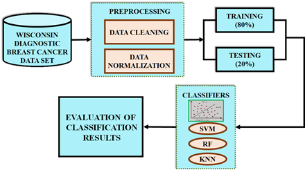
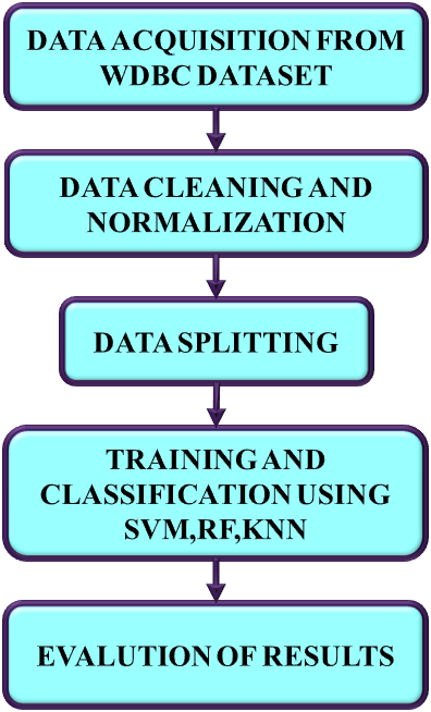
Breast cancer has emerged as one of the common diseases among women that cause death. Breast cancer is curable if diagnosed early; otherwise, it causes serious health problems and even result in the patient's death. Therefore, this paper proposes the ML approaches such as KNN, SVM and RF methods and that are analyzed for the classification of BC data. The developed block diagram is presented in Figure1(a) and process flow diagram is in Figure 1(b).
|
(a) |
|
(b) |
Figure 1. (a). Developed block diagram (b). Process flow diagram
The input data is taken from the WDBC dataset and is then subjected to a preprocessing stage that includes data normalization and cleaning. The quality, accuracy, and applicability of the input data are enhanced in this step for subsequent analysis. Next, two stages of pre-processed data are separated: training dataset and testing dataset. The training data comprises 80% of the data to build machine learning models. 20% of the data, also known as the test set / test data determines the model’s performance. This split offers the learning of underlying data patterns generating large training set, also reserving a meaningful portion of data for unbiased performance evaluation. Three machine learning approaches include KNN, RF, and SVM are employed to classify the BC data. From that, the best ML method is selected for the earliest prognosis of breast cancer based on the evaluation metrics including accuracy, precision, recall and F1-score.
Wisconsin Diagnostic Breast Cancer Dataset
This research uses the Wisconsin database for the prognoses of breast cancer. There are 212 benign entries and 357 malignant records in this unbalanced database. To address the class imbalance in the adjusting class weights in algorithms such as SVM and RF is adopted, allowing the model to give more importance to the minority class during training. Additionally, for KNN that do not directly support class weighting, stratified k-fold cross-validation is applied to preserve the class distribution across training and validation folds, ensuring fair performance evaluation. The dataset’s attributes are estimated from a digitized image of a BC sample attained from fine needle aspirate.
Preprocessing of Data
Data preprocessing converts the low-quality data to a high-quality data from WDBC dataset. It is a vital stage in converting original data into a more beneficial and understandable format for further classification purpose.
Data Cleaning
It is the initial step in filtering dataset, making it usable and readable with techniques like eliminating duplicates, managing missing values, and conversion of data type ensuring accurate and reliable results for classification.
Data Normalization
A data mining approach called min-max data normalization transforms a dataset's values into a common scale. This is crucial because many ML algorithms perform better with normalized data since they are sensitive to the input feature scale. After preprocessing, the classification of BC data is analyzed using MLmethods as KNN, SVM and RF.
Classification Using MI Algorithms
For prediction of breast cancer, three different ML algorithms are used for classifying the data.
SVM
The SVM algorithm is applied in this work as a BC prediction model that is based on statistical learning theory. The SVM algorithm develops a complex decision boundary among 2 classes with better classification abilities. The fundamental ideas of SVM are shown in Figure 2 and Figure 3. When the data cannot be separated linearly, the algorithm creates a hyper plane that divides class members from non-members as shown in Figure 3 and maps the input space using a nonlinear mapping selected a priori as depicted in Figure 2. SVM presents the idea of "margin" on both sides of the hyper plane dividing the 2 classes. It has been demonstrated that maximizing the margins will minimalize the upper bound on the expected generalization error by generating the greatest distance among the separating hyper plane and the samples on either side. SVM is considered as a linear classifier within the feature space. When classes are linearly divisible, SVM partitions them by determining the best (largest margin) separating hyper plane. One way to determine the optimal hyper plane is to solve a convex Quadratic Programming (QP) problem. Data samples that are on the edge of the ideal separation hyper plane are known as support vectors once it has been identified. This optimization issue has a global solution.
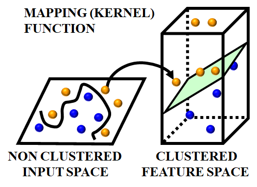
Figure 2. Input space mapping without clustering to a higher dimensional feature space
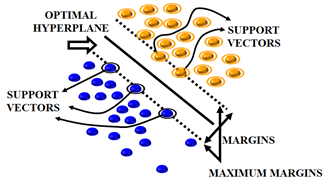
Figure 3. Optimal hyper plane splitting the classes and support vectors
Assume that the training subset for a linearly decision space has  samples
  and
and  , meaning that data only have 2 classes. The separating hyper plane is:
| 
| (1) |
Where training subset of linearly separable data is used to learn the vector  and constant
 . For both targets with y equal to (-1) and (1), the SVM solution is equal to solving a linear restricted quadratic programming problem using Equation (2):
| 
| (2) |
The support vectors are samples that, in the event of equality, give the Equation (2). The samples are classified by SVM with these support vectors. Conversely, the hyper plane's margins obey the following inequality in equation (3):
| 
| (3) |
To increase the margin  , the norm ofis need to be diminished. The following equation is supposed to decrease the number of results to norm of .
| 
| (4) |
Next, the algorithm, considers the parameters in Equation (2), attempts to minimalize the value of  . When dealing with slack parameters
 , non-separable samples are introduced into Equation (2) in the subsequent manner:
| 
| (5) |
The slack variables are introduced to allow some samples to violate the ideal margin, meaning the model can tolerate some misclassification or margin violations. To train the SVM under these relaxed constraints, the goal becomes two-fold including minimizing the margin width and minimizing the total penalty from margin violations. These two objectives are combined into a single optimization function in equation (6).
| 
| (6) |
Where the regularization parameter is  and that is known as the cost parameter, allow for larger deviations from the ideal solution with greater values. They also serve as a measure of the model's tolerance. This parameter is tuned to attain a concession among the model's complexity and classification error. Input space is mapped into feature space using a variety of kernel functions. They start with basic mappings of sigmoid and radial basis functions that are linear and polynomial. SVM employs this function to map novel samples into the feature space for classification after a hyper plane has been generated. Unlike other ML approaches, SVM is made dimensionally independent by this mapping method. In this article, the input space is mapped into a higher dimensional feature space utilizing Radial Basis Function (RBF) kernel. So, just one parameter that needs to be optimized for RBF kernels: the width of the basic functions
 . The RBF kernel's width is detected by a positive real number (
 ) and is given in equation (7).
| 
| (7) |
Tuning of the SVM model, particularly the parameter of the RBF kernel and the regularization parameter , is performed using a grid search combined with cross-validation. In this process, a predefined set of values for both and are tested across different combinations to identify the pair that resulted in the highest classification accuracy on the validation set. During grid search, multiple folds of the training data are used in a k-fold cross-validation setting to ensure that the selected hyperparameters generalized well across different subsets. The combination of and that yielded the best average performance is then chosen to train the final SVM model. This tuning process helps prevent overfitting and ensures that the model performs robustly on unseen test data. The RBF kernel is chosen for SVM because it is highly effective in handling non-linear relationships between features, which are common in medical datasets like WDBC. Unlike the linear kernel, which assumes a straight-line decision boundary, the RBF kernel enables capturing complex patterns. Compared to the polynomial kernel, the RBF kernel requires fewer hyperparameters, reducing the risk of overfitting and making it more computationally efficient and easier to tune.
RF
The RF classifier serves as an ensemble learning technique and used as a prediction model for breast cancer. RF employs bootstrap sampling approach to obtain many distinct training subsets from the original training set. In the RF algorithm, feature randomness and ensemble aggregation work together to enhance model accuracy and generalization. Feature randomness is introduced during the construction of each decision tree: at every split in a tree, only a random subset of features ( ) is considered rather than evaluating all available features. This process reduces correlation among individual trees and encourages diversity in their structure, which helps in reducing overfitting. Additionally, ensemble aggregation is achieved by building multiple such trees and combining their predictions through a majority voting strategy for classification tasks. Each tree contributes a vote to the final decision, and the class with the most votes is selected as the model’s output. All training subsets are used to train a decision tree and it eventually produce a RF. Each tree's vote counts toward the final forecast for a binary task. The exact method of RF is displayed in Figure 4. Step 1: Choose
  samples from training set by using the Bootstrap approach. Step 2: Choose features arbitrarily and the decision tree node is split using the least Gini value with feature. Step 3: To obtain
  decision trees, repeat steps 1 and 2 a total of times. Step 4: Create a random forest by combining the decision trees, and ascertain voting-based classification outcome.
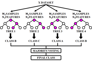
Figure 4. Random forest model
KNN
KNN shown in Figure 5 is a simple classifier whose effectiveness is determined by the value chosen and the similarity metrics (distance functions) applied. KNN classifier is a popular method for differentiating healthy and sick instances after selecting attributes. Nonetheless, it also produce competitive results, and in certain instances. Every unknown occurrence in the training set is classified by the KNN rule based on a majority marking among its closest KNN neighbors.
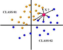
Figure 5. The KNN method
The distance metric used to identify the closest neighbors has an impact on its performance. In the absence of prior information, the majority of KNN classifiers quantify the difference between samples given as vector inputs using basic Euclidean metrics. Using the Equation (8), the Euclidean distance is computed.
| 
| (8) |
When a vector  is used to describe an example, is the input vector's dimensionality, or the quantity of sample attributes. An example attribute is
  and its weight
  ranges from
  , smaller
 indicates which of the two examples is more pertinent.
| 
| (9) |
In this case  represents a test and is one of the training set's closest neighbors,
  indicates whether
  relates to class
  . According to equation (9), the class that has the majority of its members in the nearest k neighbors is the predictor.
KNN Algorithm Steps
- Enter the data set and divide it into testing and training sets.
- Select an instance from the test sets and estimate how distant it is from the training set.
- Enumerate the distances in increasing order.
- In the first three training instances
 , the instance's class is the most specialized class.
Specifically, k-fold cross-validation is applied, and during this process, various values of k are tested, and their corresponding classification accuracies are recorded. The value of k that results in the highest average validation accuracy across all folds is selected as the optimal number of neighbours. The performance of KNN has a significant impact on the measure utilized to determine the distances between the instances.
- RESULTS AND DISCUSSION
This paper proposes the ML algorithms including SVM, RF and KNN for breast cancer identification. To ensure the high quality of data, the work adopts preprocessing step that includes data cleaning and normalization. After preprocessing, the ML algorithms are analyzed for the classification of BC data. The developed work is implemented in python software and comparative analysis is done with traditional methods to show the superior performance of the developed work. Figure 6 shows the diagnosis count plot and pie chart of breast cancer. Number 0 represents the benign breast cancer, whereas number 1 represents the malignant type. There are 357 number of benign BC and 212 cases of malignant BC (total=569 samples).
Figure 7 indicates a correlation matrix where each value in the dataset is depicted by a different colour and it helps to identify highly correlated features. Its features contain radius, texture, perimeter, area, smoothness, compactness, concavity, etc. of BC data. When there is a significant correlation between two features, the classifier's performance is affected. The strong positive correlation between features such as radius_mean, perimeter_mean, and area_mean, with correlation values close to 1.0, indicating a high degree of linear relationship among them. Specifically, the high correlation between radius and perimeter suggests that these features may be redundant, as they convey overlapping information.
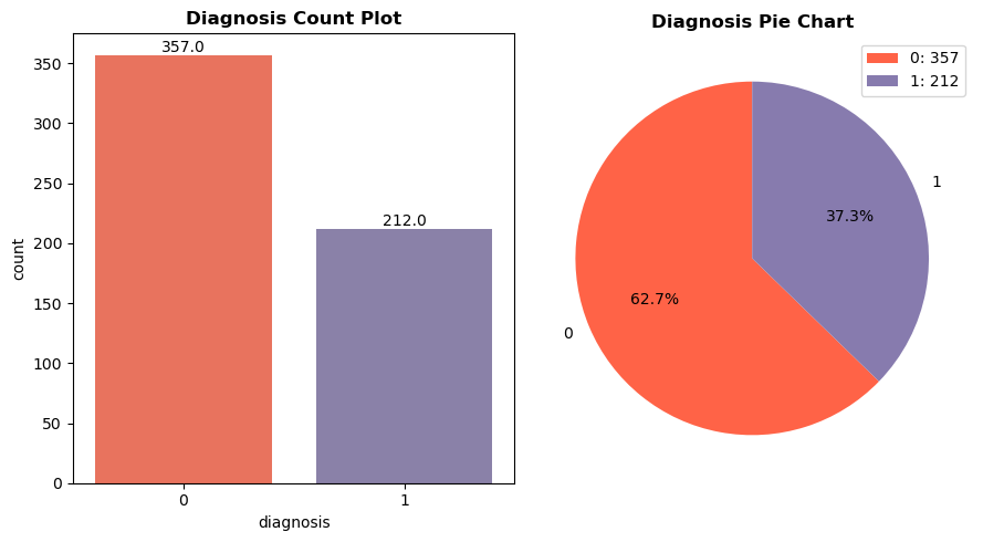
Figure 6. Diagnosis count
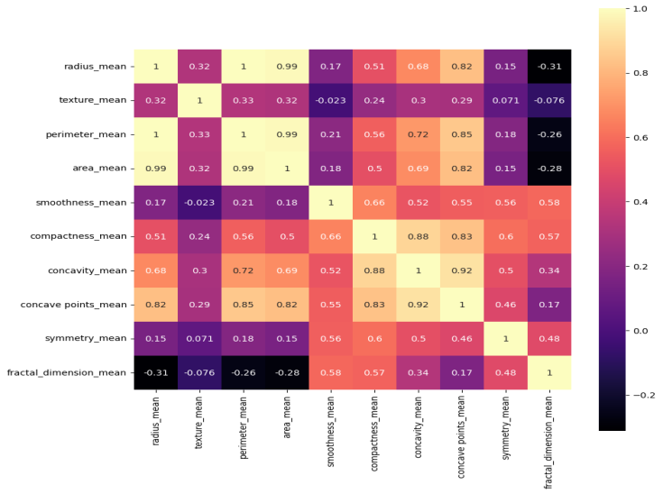
Figure 7. Correlation matrix
The distribution plots of the various attributes from the chosen dataset used in this work are displayed in Figure 8. It provides the distribution of different features with benign and malignant tumor types that is mainly utilized to detect the breast cancer. Figure 9(a), Figure 9(b), and Figure 9(c) highlights the confusion matrix for RF, SVM, and KNN, which is an indication of matrix of the prediction summary. It shows the number of accurate and inaccurate forecasts for each class. The confusion matrix of KNN has highly accurate predicted values, which proves KNN outperforms than other ML methods. It helps reduce such misclassifications by learning from patterns in historical data, ultimately supporting more reliable and earlier detection of breast cancer, which is vital for improving patient outcomes. Figure 10(a) and Figure (b) show the Receiver Operating Characteristics (ROC) and precision-recall curve for RF, SVM, and KNN. It is evident from Figure 10 that KNN has an AUC value of 0.953 and a precision-recall of 0.942, which is better than RF and SVM methods. SVM has an AUC value of 0.930 and a precision-recall of 0.913, RF has an AUC value of 0.946 and a precision-recall of 0.919. The high ROC-AUC and Precision-Recall values observed for KNN, despite the class imbalance is due to the effective data preprocessing, careful parameter tuning and robust evaluation methods used in the proposed approach. Specifically, normalization and noise reduction during preprocessing helped ensure KNN is not biased by scale variations in features. Additionally, the use of k-fold cross-validation helped maintain representative distributions of both classes across folds, preventing skewed evaluation.
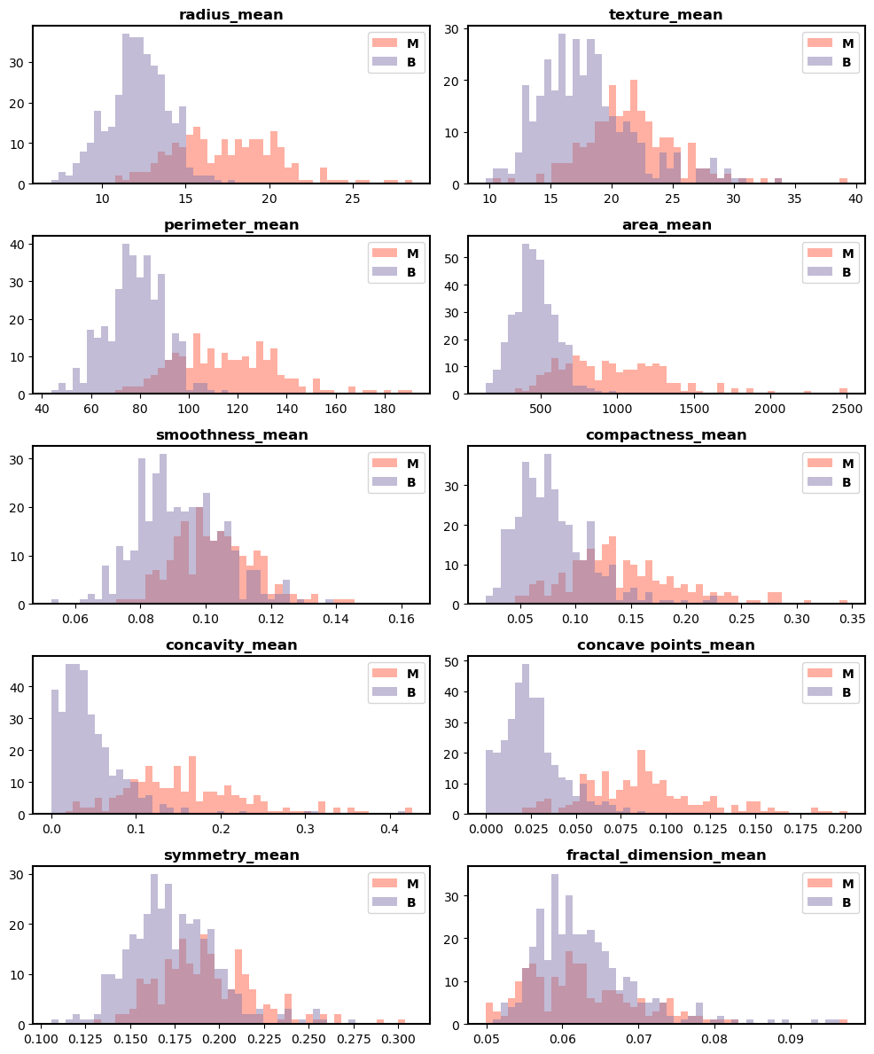
Figure 8. Distribution plots of different attributes
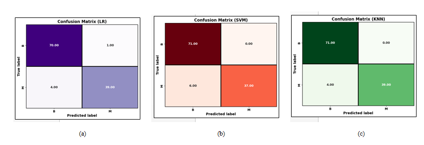
Figure 9. Confusion matrix for (a) RF (b) SVM (c) KNN
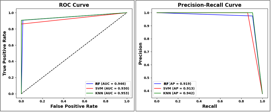
Figure 10. (a) ROC graph (b) Precision-Recall graph for RF, SVM and KNN
The comparison of performance metrics for ML algorithms such as RF, SVM, and KNN is displayed in Table 1. The KNN method has the maximum accuracy and F1-score value of 96.49% and 95.12%, compared to the RF and SVM methods. The recall value is the same and higher for RF and KNN than SVM, and the precision value is the same and higher for SVM and KNN than RF method. Table 2 presents a comparison of the training time required by RF, SVM and KNN. KNN exhibits the shortest training time of just 0.01 seconds, SVM requires a moderate training time of 0.30 seconds and RF has the longest training time at 0.50 seconds. Accuracy is the proportion of total correct predictions made by the model out of all predictions. The accuracy comparison for MLP [25], NB [26] and the developed ML methods are shown in Figure11. The developed KNN outperforms (accuracy of 96.49%) than the MLP, NB and the proposed RF and SVM method. Specificity measures the proportion of actual negative cases correctly identified by the model. Figure 12 represents the specificity comparison with MLP [27], Adaboost [28] and the ML algorithms. The proposed KNN attains the higher specificity value of 94.8% compared to other methods. F1-score indicates harmonic mean of recall and precision, considering both false negatives and false positives. The comparison of F1-scorewith DT [29], Adaboost [30] and ML algorithms is highlighted in Figure 13. The proposed KNN has highest F1-score of 95.12% that is better than other methods (DT, Adaboost, SVM and RF). KNN makes no assumptions about data distribution and directly classifies sample depending on the majority class among its closest neighbours. This characteristic proves advantageous in the WDBC dataset, where classes may not be linearly separable, and subtle variations in feature values can strongly indicate tumor type. Moreover, with well pre-processed data and an appropriately chosen value of K through cross-validation, KNN provides high accuracy and robustness without the complexity of model training.
Table 1. Comparison of evaluation metrics
Classifiers | Accuracy | Recall | Precision | F1-score |
RF | 95.6% | 90.7% | 97.5% | 93.9% |
SVM | 94.7% | 86.1% | 100.0% | 93.9% |
KNN | 96.5% | 90.7% | 100.0% | 95.1% |
Table 2. Comparison of training time
Classifiers | Training time (s) |
RF | 0.50 |
SVM | 0.30 |
KNN | 0.01 |
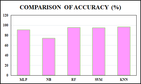
Figure 11. Comparison of accuracy
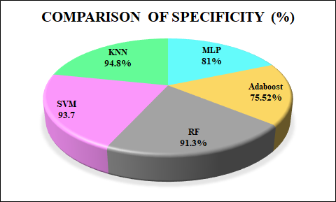
Figure 12. Specificity comparison
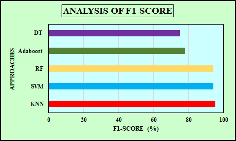
Figure 13. F1-score comparison
- CONCLUSIONS
A ML algorithm based approach for detecting breast cancer is developed in this research. The data is acquired from WDBC dataset and classification techniques are applied to separate and classify tumor types, or benign and malignant cells. Data preprocessing (cleaning, normalization) enhances input quality. After preprocessing, the ML methods such as KNN, SVM and RF methods are analyzed for the classification of data. We implemented the work in python software and comparative analysis is made with conventional methods like MLP, NB, DT. It is confirmed that KNN has the better performance metrics than other ML algorithms with an accuracy of 96.49%, recall of 90.7%, F1-score of 95.12% and specificity of 94.8%. Its ability to learn from local structures in the data and its tolerance to overlapping class boundaries contributes to its superior classification performance in this context. Since KNN has demonstrated high classification accuracy, particularly in identifying subtle patterns in diagnostic features, it enhances the reliability of automated screening tools. This leads to faster clinical decisions, reduced diagnostic delays and earlier intervention, all of which are vital for increasing survival rates and reducing treatment complexity. Despite the promising results achieved in this study, there are certain limitations that warrant attention. Firstly, the model performance is evaluated solely on the WDBC dataset, which may limit its generalizability to other datasets or real-world clinical scenarios with more complex and varied data. Additionally, the study focuses on only three classifiers excluding more advanced or ensemble-based methods that could potentially yield higher accuracy and robustness. For future research, the methodology can be extended by incorporating larger, more diverse datasets, including real-time clinical data. Exploring deep learning models as well as hybrid or ensemble learning techniques may improve classification performance.
DECLARATION
Acknowledgement
Not Applicable.
Conflicts of Interest
An authors have no conflicts of interest to declare that are relevant to the content of this article.
REFERENCES
- Y. S. Solanki, P. Chakrabarti, M. Jasinski, Z. Leonowicz, V. Bolshev, A. Vinogradov, E. Jasinska, R. Gono, and M. Nami, “A hybrid supervised machine learning classifier system for breast cancer prognosis using feature selection and data imbalance handling approaches,” Electronics, vol. 10, pp. 699, 2021, https://doi.org/10.3390/electronics10060699.
- S. Yadav, and M. Shivajirao, “Thermal infrared imaging based breast cancer diagnosis using machine learning techniques,”Multimedia Tools and Applications, vol. 81, pp. 1-19, 2022, https://doi.org/10.1007/s11042-020-09600-3.
- K. M. M. Uddin, N. Biswas, S. T. Rikta, and S. K. Dey, “Machine learning-based diagnosis of breast cancer utilizing feature optimization technique,” Computer Methods and Programs in Biomedicine Update, vol. 3, pp. 100098, 2023, https://doi.org/10.1016/j.cmpbup.2023.100098.
- A. S. Assiri, S. Nazir, and S. A. Velastin, “Breast tumor classification using an ensemble machine learning method,” Journal of Imaging, vol. 6, pp. 39, 2020, https://doi.org/10.3390/jimaging6060039.
- J. Wu, and C. Hicks, “Breast cancer type classification using machine learning,” Journal of personalized medicine, vol. 11, pp. 61, 2021, https://doi.org/10.3390/jpm11020061.
- R. Rawal, “Breast cancer prediction using machine learning,” Journal of Emerging Technologies and Innovative Research (JETIR), vol. 13, pp. 7, 2020, https://www.jetir.org/view?paper=JETIR2005145.
- M. A. Naji, S. El Filali, K. Aarika, E. H. Benlahmar, R. A. Abdelouhahid, and O. Debauche, “Machine learning algorithms for breast cancer prediction and diagnosis,” Procedia Computer Science, vol. 191, pp. 487-492, 2021, https://doi.org/10.1016/j.procs.2021.07.062.
- P. Gupta, and S. Garg, “Breast cancer prediction using varying parameters of machine learning models,”Procedia Computer Science, vol. 171, pp. 593-601, 2020, https://doi.org/10.1016/j.procs.2020.04.064.
- A. Khalid, A. Mehmood, A. Alabrah, B.F. Alkhamees, F. Amin, H. AlSalman, and G. S. Choi, “Breast cancer detection and prevention using machine learning,” Diagnostics, vol. 1319, pp. 3113, 2023, https://doi.org/10.3390/diagnostics13193113.
- O. Díaz, A. Rodríguez-Ruíz, and I. Sechopoulos, “Artificial Intelligence for breast cancer detection: Technology, challenges, and prospects,” European journal of radiology, vol. 175, pp. 111457, 2024, https://doi.org/10.1016/j.ejrad.2024.111457.
- L. Wang, “Mammography with deep learning for breast cancer detection,” Frontiers in oncology, vol. 14, pp. 1281922, 2024, https://doi.org/10.3389/fonc.2024.1281922.
- S. Sushanki, A. K. Bhandari, and A. K. Singh “A review on computational methods for breast cancer detection in ultrasound images using multi-image modalities,” Archives of Computational Methods in Engineering, vol. 31, no. 3, pp. 1277-1296, 2024, https://doi.org/10.1007/s11831-023-10015-0.
- S. A. Alanazi, M. M. Kamruzzaman, M. N. Islam Sarker, M. ARFuwaili, Y. Alhwaiti, N. Alshammari, and M. H. Siddiqi, “Boosting breast cancer detection using convolutional neural network,” Journal of Healthcare Engineering, vol. 1, pp. 5528622, 2021, https://doi.org/10.1155/2021/5528622.
- A. Das, M. N. Mohanty, P. K. Mallick, P. Tiwari, K. Muhammad, and H. Zhu, “Breast cancer detection using an ensemble deep learning method,”Biomedical Signal Processing and Control, vol. 70, pp. 103009, 2021, https://doi.org/10.1155/2021/5528622.
- U. Naseem, J. Rashid, L. Ali, J. Kim, Q.E.U. Haq, M.J. Awan, and M. Imran, “An automatic detection of breast cancer diagnosis and prognosis based on machine learning using ensemble of classifiers,” IEEE Access, vol. 10, pp.78242-78252, 2022, https://doi.org/10.1109/ACCESS.2022.3174599.
- I. Hirra, M. Ahmad, A. Hussain, M. U. Ashraf, I. A. Saeed, S. F. Qadri, A. M. Alghamdi, and A. S. Alfakeeh, “Breast cancer classification from histopathological images using patch-based deep learning modeling,” IEEE Access, vol. 9, pp. 24273-24287, 2021, https://doi.org/10.1109/ACCESS.2021.3056516.
- H. Aljuaid, N. lturki, N. Alsubaie, L. Cavallaro, and A. Liotta, “Computer-aided diagnosis for breast cancer classification using deep neural networks and transfer learning,” Computer Methods and Programs in Biomedicine, vol. 223, pp. 106951, 2022, https://doi.org/10.1016/j.cmpb.2022.106951.
- B. O. Macaulay, B. S. Aribisala, S. A. Akande, B. A. Akinnuwesi, and O. A. Olabanjo, “Breast cancer risk prediction in African women using random forest classifier,” Cancer Treatment and Research Communications, vol. 28, pp. 100396, 2021, https://doi.org/10.1016/j.ctarc.2021.100396.
- Z. Huang, and D. Chen, “A breast cancer diagnosis method based on VIM feature selection and hierarchical clustering random forest algorithm,” IEEE Access, vol. 10, pp. 3284-3293, 2021, https://doi.org/10.1109/ACCESS.2021.3139595.
- P. Manikandan, U. Durga, and C. Ponnuraja, “An integrative machine learning framework for classifying SEER breast cancer,” Scientific Reports, vol. 13, pp. 5362, 2023, https://doi.org/10.1038/s41598-023-32029-1.
- M. Liu, L. Hu, Y. Tang, C. Wang, Y. He, C. Zeng, K. Lin, Z. He, and W. Huo, “A deep learning method for breast cancer classification in the pathology images,” IEEE Journal of Biomedical and Health Informatics, vol. 26, pp. 5025-5032, 2022, https://doi.org/10.1109/JBHI.2022.3187765.
- R. G. Babu, K. Dhineshkumar, R. Sharma, and R. Krishnamoorthy, “A survey of machine learning techniques using for image classification in home security,” In IOP Conference Series: Materials Science and Engineering, vol. 1055, pp. 012088, 2021, https://doi.org/10.1088/1757-899X/1055/1/012088.
- X. Y. Liew, N. Hameed, and J. Clos, “An investigation of XGBoost-based algorithm for breast cancer classification,” Machine Learning with Applications, vol. 6, pp. 100154, 2021, https://doi.org/10.1016/j.mlwa.2021.100154.
- K. Satish Kumar, V. V. S. Sasank, K. S. Raghu Praveen, and Y. Krishna Rao, “Multilayer perceptron back propagation algorithm for predicting breast cancer,” In Intelligent System Design. Proceedings of Intelligent System Design, pp. 41-53, 2021, https://doi.org/10.1007/978-981-15-5400-1_5.
- Z. Guo, L. Xu, and N. Ali Asgharzadeholiaee, “A homogeneous ensemble classifier for breast cancer detection using parameters tuning of MLP neural network,” Applied Artificial Intelligence, vol. 36, no. 1, pp. 2031820, 2022, https://doi.org/10.1080/08839514.2022.2031820.
- M. Mangukiya, A. Vaghani, and M. Savani, “Breast cancer detection with machine learning,” International Journal for Research in Applied Science and Engineering Technology, vol. 10, no. 2, pp. 141-145, 2022, https://doi.org/10.22214/ijraset.2022.40204.
- M. A. Elsadig, A. Altigani, and H. T. Elshoush, “Breast cancer detection using machine learning approaches: a comparative study,” International Journal of Electrical & Computer Engineering, vol. 13, no. 1, pp. 2088-8708, 2023, https://doi.org/10.11591/ijece.v13i1.pp736-745.
- Y. K. Qawqzeh, A. Alourani, and S. Ghwanmeh, “An improved breast cancer classification method using an enhanced AdaBoost classifier,” International Journal of Advanced Computer Science and Applications, vol. 14, no. 1, 2023, https://doi.org/10.14569/IJACSA.2023.0140151.
- M. M. Ghiasi, and S. Zendehboudi, “Application of decision tree-based ensemble learning in the classification of breast cancer,” Computers in biology and medicine, vol. 128, pp. 104089, 2021, https://doi.org/10.1016/j.compbiomed.2020.104089.
- S. Gamil, F. Zeng, M. Alrifaey, M. Asim, and N. Ahmad, “An efficient AdaBoost algorithm for enhancing skin cancer detection and classification,” Algorithms, vol. 17, no. 8, pp. 353, 2024, https://doi.org/10.3390/a17080353.
Vanitha M (Effective Analysis of Machine Learning Algorithms for Breast Cancer Prediction)