ISSN: 2685-9572 Buletin Ilmiah Sarjana Teknik Elektro
Vol. 7, No. 3, September 2025, pp. 554-571
Understanding Time Series Forecasting: A Fundamental Study
Furizal 1, Alfian Ma’arif 2, Kariyamin 3, Asno Azzawagama Firdaus 4, Setiawan Ardi Wijaya 5,
Arman Mohammad Nakib 6, Ariska Fitriyana Ningrum 7
1 Department of Research and Development, Peneliti Teknologi Teknik Indonesia, Sleman 55281, Indonesia
2 Department of Electrical Engineering, Universitas Ahmad Dahlan, Yogyakarta, 55191, Indonesia
3 Department of Information Technology, Institut Teknologi dan Bisnis Muhammadiyah Wakatobi, 93795, Indonesia
4 Department of Computer Science, Universitas Qamarul Huda Badaruddin Bagu, Central Lombok 83371, Indonesia
5 Department of Information System, Universitas Muhammadiyah Riau, Pekanbaru, 28294, Indonesia
6 School of Artificial Intelligence, Nanjing University of Information Science and Technology, Nanjing, Jiangsu, China
7 Department of Data Science, Universitas Muhammadiyah Semarang, Semarang, 50273, Indonesia
ARTICLE INFORMATION |
| ABSTRACT |
Article History: Received 22 April 2025 Revised 23 June 2025 Accepted 27 September 2025 |
| 
Time series forecasting plays a vital role in economics, finance, engineering, etc., due to its predictive power based on past data. Knowing the basic principles of time series forecasting enables wiser decisions and future optimization. Despite its importance, some researchers and professionals find it difficult to use time series forecasting techniques effectively, especially with complex data settings and selection of methods for a particular problem. This study attempts to explain the subject of time series forecasting in a comprehensive and simple manner by integrating the main stages, components, preprocessing steps, popular forecasting models, and validation methods to make it easier for beginners in the field of study to understand. It explains the important components of time series data such as trend, seasonality, cyclical components, and irregular components, as well as the importance of data preprocessing steps, proper model selection, and validation to achieve better forecasting accuracy. This study offers useful material for both new and experienced researchers by providing guidance on time series forecasting techniques and approaches that will help in enhancing the value of decision making. |
Keywords: Time Series; Forecasting; Fundamental Study; Data Preprocessing; Timestep; Validation |
Corresponding Author: Alfian Ma’arif, Department of Electrical Engineering, Universitas Ahmad Dahlan, Yogyakarta, 55191, Indonesia. Email: alfianmaarif@ee.uad.ac.id |
This work is open access under a Creative Commons Attribution-Share Alike 4.0 
|
Document Citation: F. Furizal, A. Ma’arif, K. Kariyamin, A. A. Firdaus, S. A. Wijaya, A. M. Nakib, and A. F. Ningrum, “Understanding Time Series Forecasting: A Fundamental Study,” Buletin Ilmiah Sarjana Teknik Elektro, vol. 7, no. 3, pp. 554-571, 2025, DOI: 10.12928/biste.v7i3.13318. |
INTRODUCTION
Time series forecasting is an indispensable analytical technique for predicting unknown future events using past data [1][2]. It is used by various disciplines such as economics, finance, marketing, and supply chain management [3]. It evaluates trends, seasonality, cycles, and other time-related patterns to help organizations and researchers formulate informed decisions [4]. The advent of Artificial Intelligence (AI) technology [5] has simplified time series forecasting and improved models in terms of accuracy and agility. The complex nature of time series data poses many challenges, especially for novice forecasters [6]. Understanding these challenges and approaches is essential to ensure precise forecasting and decision making. Despite its relevance, many academics and professionals, especially novices, find it difficult to perform time series forecasting techniques. The data is often noisy [7][8] and contains irregular shifts and missing values that mask certain patterns. Furthermore, the simpler ARIMA [9] and Exponential Smoothing models, which are reasonable with some data, are not applicable to more advanced non-linear problems. This makes it difficult to select the most appropriate method for different types of time series data, increasing the likelihood of errors in forecasting.
This problem is still unsolved because it deals with time series data, which is quite complex. Sometimes, time series data can have trends, seasonality, cyclical behavior, etc., all of which require different forecasting models. Moreover, the complexity of real-world data sets tends to be sophisticated [10][11], for example, they may have missing values or outliers, which are very difficult for beginners to understand. Moreover, a lot of time is needed to clean the data, choose the right model, and validate it. Most beginners do not have these various forecasting techniques, making the whole process daunting. Simply put, researchers who want to solve time series forecasting problems can get lost due to the lack of a clear framework to work with.
In this study, the authors propose to design a simple and easy-to-follow time series forecasting guide that offers a step-by-step approach. This approach attempts to assist beginners in the field of time series forecasting by breaking down the process into less complex steps, starting with data preprocessing, then model selection, and ending with validation techniques. These methods will enable practitioners and researchers to understand not just isolated techniques, but the entire system as a cohesive unit that improves forecast accuracy. Thus, the contribution of this study is to propose a coherent and concise description of the steps involved in the time series forecasting process that will help researchers, especially beginners, in understanding and utilizing the methodology, thereby producing better and more reliable results.
- WHAT IS TIME SERIES FORECASTING?
Time series data consists of a series of values recorded over a period of time, such as stock prices or daily temperatures [12][13]. This data allows us to study patterns that have occurred over a period of time to understand how values change over time [14][15]. By analyzing time series data, it is possible to understand the relationships that exist between multiple time factors of an event, which in turn helps in understanding how past conditions have influenced the current state. This data allows us to project the detected patterns into the future, which will support planning and anticipating future changes. The method used to predict future values from a time-mapped dataset and the historical data used is known as time series forecasting [16]-[18]. When the data is readily available and well organized, the forecasting process becomes easier and faster. This technique is essential for sales forecasting, stock evaluation, and planning organizational activities. Relying on past data allows an organization to plan more effectively and understand what changes are likely to occur in the future.
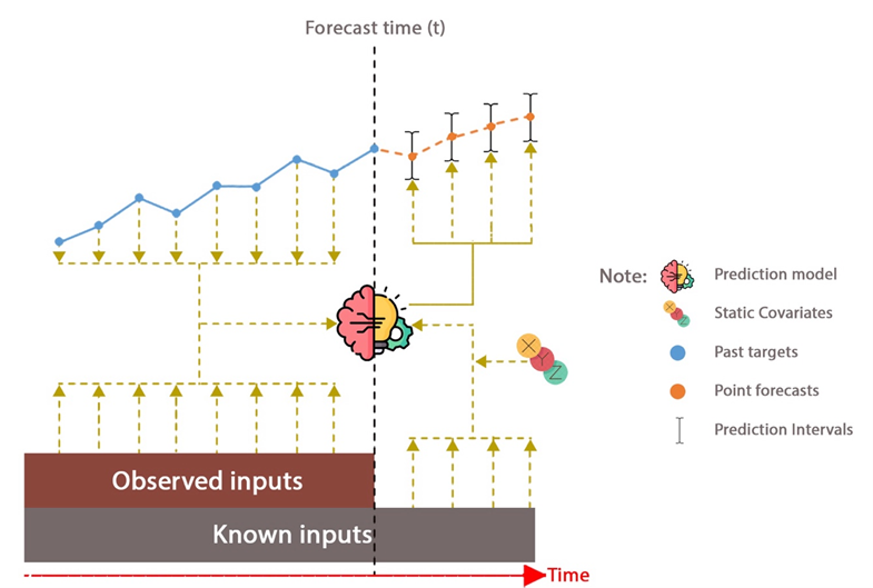
Although time series forecasting can provide useful predictions, the results are not always completely accurate [19][20]. Uncertainty and unforeseen external factors, such as sudden events or radically changing market conditions, affect forecast accuracy. Despite its imperfections, time series forecasting still offers insight into possible future outcomes, which helps organizations make better decisions. While it is impossible to completely eliminate uncertainty, time series forecasting serves as an important tool during the decision-making process and strategic planning. In time series forecasting, the model used attempts to recognize and exploit identifiable patterns in historical data, to predict how variables will change in the future [21][22]. The temporal order of the data is critical because future values often depend on past values. If there is an upward or downward trend in the data, the model must be able to exploit that trend and predict similar value movements in the future. An illustration of the time series forecasting process is shown in Figure 1.
Figure 1 illustrates a multi-horizon (time series-based) forecasting method that is able to predict values for several periods in the future, while considering multiple data sources simultaneously [23][24]. The model combines historical data (past targets), directly observed inputs (observed inputs), known information (known inputs), plus constants called static covariates. By considering these components, the model tends to capture patterns of trends, seasonality, and fluctuations in the data, thereby increasing forecast accuracy. Past targets provide the necessary information on the history of the variable to be predicted and help the model to capture temporal changes. On the other hand, observed inputs include factors that have been observed and may affect the target such as environmental, economic, or social factors. By incorporating observed inputs, the model can account for changes that are not always detected through historical data.
Known inputs consist of variables that are known at the time of the forecast such as public holiday calendars, production schedules, or even deterministic external data. The presence of known inputs allows the model to better recognize the presence of deterministic patterns, resulting in more accurate and stable predictions. Static covariates are parameters that do not change over the forecast period, such as geographic location, product type, or customer demographics. This allows the model to capture patterns that are specific to the idiosyncratic characteristics of the entity being analyzed. After processing all of these inputs, the model produces a set of forecasts for a number of future periods, with prediction intervals that describe how uncertain the estimates are.
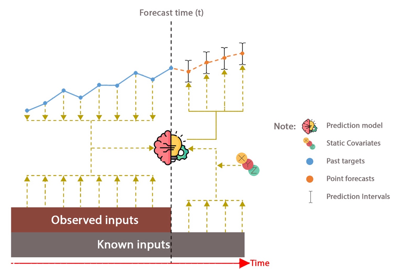
Figure 1. Illustration of the time series forecasting process [23][24]
- GENERAL STAGES IN TIME SERIES FORECASTING
Forecasting is the process of making predictions or decisions that can predict the future [25][26]. The first step involves developing objectives. This is where the forecast objective is set along with the appropriate figures and time frame. It is important to understand whether the scope is built for short-term operational decisions, medium-term planning, or long-term strategic insights as this determines the methods and data to be used. Forecasting without accurate and intelligent objectives cannot produce results and decisions that can be helpful, rather than unconstructively misleading. Once the specific objectives are clearly defined, the next step is to obtain relevant data. Point-in-time data, such as sensor readings, sales information, and market trends, provide the essence of any forecast. However, the data used must still be appropriate and relevant to the research objectives. It is essential that the data collection process ensures that the data is accurate, uncorrupted, and complete as any missing values or errors can result in incorrect forecasts. As such, data must be cleaned and validated before it is subjected to analysis.
When analyzing data, it is often necessary to pre-process it. This involves data cleaning, which includes removing noise, handling outliers, imputing missing or duplicate values, handling multiple repeating records, and several other preprocessing steps to ensure that the data is ready to be processed by the forecasting model [27]-[30]. A data set can be considered fully reliable for forecasting only after thorough cleaning, structuring, and fine-tuning have been applied (more clearly discussed in section: VI. Data Preprocessing in Time Series Forecasting). Once the data is prepared, the next challenge is to choose the right forecasting method. Forecasting can be done using qualitative or quantitative techniques. Qualitative methods, such as opinion surveys and the Delphi technique, are generally used when the data is scarce, and expert judgment is required. On the other hand, quantitative methods—such as ARIMA (Auto Regressive Integrated Moving Average) [31], exponential smoothing [32], regression models [32], and even machine learning algorithms [33][34], are preferred when large data sets are available (more clearly discussed in section: VII. Popular Method for Time Series Forecasting). These methods take into account the time-dependent nature of the data, incorporating patterns such as seasonality, trends, and cycles. The method chosen depends on the characteristics of the data, the complexity of the forecast required, and other constraints.
Once the approach method is determined, data analysis begins with an attempt to highlight identifiable patterns, trends, and relationships. This is a very important step, as it incorporates everything from seasonal effects to related cyclical variations that seem to affect the forecast. To provide further clarity on the predictions, statistical techniques are accompanied by data visualization tools to identify patterns and factors that help make the predictions more accurate. The analysis is so thorough that one can be sure that any forecast made will take into account as many factors as possible and contain very few risks. In relation to the information collected, the actual forecasting process begins. Before proceeding with the forecasting process, the method is first trained using historical data to recognize the patterns contained therein. This training process then produces a model that will be used for the forecasting process. To find out how reliable the model is, validation is needed (more clearly discussed in section: VIII. Validating Time Series Forecasting Results). The validation process is an integral part of estimating the accuracy of the forecast. Comparing the forecast with its actual value allows the analyst to evaluate the accuracy of the forecast using various error indices. The level of forecast discrepancy often requires a reality check, where the model is iteratively improved to achieve the desired level of accuracy. The process of revising and refreshing the model with new data maintains the accuracy and usefulness of the predictions. As organizations improve their forecasting approaches, they hope to achieve greater readiness and adaptability to environmental changes. Some common stages in time series forecasting from defining objectives to achieving objectives are shown in Figure 2.
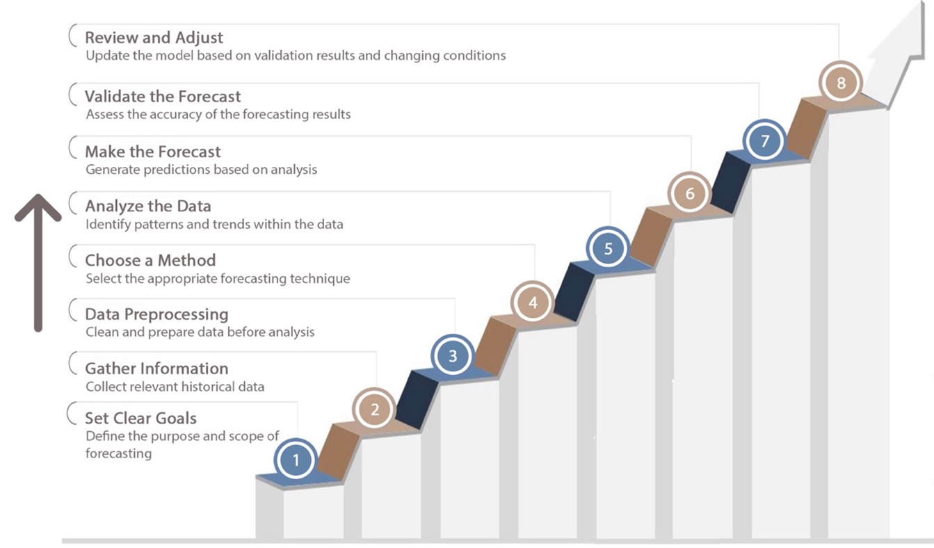
Figure 2. General stages of the time series forecasting process from determining goals to obtaining the desired goals
- TIMESTEP DALAM TIME SERIES FORECASTING
Time step in the context of forecasting refers to a specific time interval or period used to predict future values in a time series, based on previous data. Time step refers to the unit of time used to measure the distance between two consecutive data points in a time series. For example, in a time series that records daily temperatures, the time step is one day, indicating that data is collected every 24 hours. Time steps can vary, depending on the data being analyzed, such as weekly, monthly, or even yearly [35][36]. In the context of forecasting, time steps are used to predict future values based on historical data and patterns identified in that data [25][26]. It is important to remember that in time series forecasting, it is not only predictions at a specific point in time that are needed, but also how those predictions are influenced by previous time steps. Time step forecasting uses patterns formed from a series of data to predict future values, so patterns or trends that emerge in historical data can be used to project future conditions.
Single-step Forecasting
Single-step forecasting is an analysis that focuses on anticipating a single future value based on available information [37][38]. The model’s predictions are limited to a single time period, or one step ahead, usually referred to as t+1, which is the next period after the last data point. This method is relatively easy to implement and is appropriate for cases where only a single time unit projection is needed. For example, in sales forecasting, if the only question is what the sales figures will be in the next month (t+1), then single-step forecasting is sufficient. The forecasting model will base its estimates on historical data from several previous periods, perhaps covering sales for the past month and several months before that. This approach is most useful when the desired information is relevant to only one future time period, as shown in Figure 3(b). However, a disadvantage of single-step forecasting is that it does not account for changes or trends that may occur more than one time step ahead. This makes this approach unsuitable for long-term projections that require multiple time steps ahead.
Multi-steps Forecasting
Multi-step forecasting refers to a more advanced approach to forecasting where the primary objective is to predict more than one value in a time series in the future [39]-[41]. Instead of predicting the value for just one time period such as t+1, multi-step forecasting is a model that attempts to make predictions for multiple time periods simultaneously; for example, the objective may include making forecasts for t+1, t+2, t+3, .. up to t+n, which also includes projections for multiple time periods at once. This method is very useful in many cases, especially where details about longer-term future conditions are important, for example, when dealing with production planning or weather forecasting, we want to know not only the value for the next period but also how the value will evolve over several future periods. Thus, multi-step forecasting models become important when one wants to get a more detailed view of expected future trends, especially in the long term. The most difficult but most significant problem with multi-step forecasting is that the further out the prediction is made, the higher the degree of uncertainty and the potential for prediction errors. This problem occurs because the model must consider a larger set of variables, along with their dependencies from one time step to another, which can result in accumulated errors.
Recursive Multi-Step Forecasting
In recursive multi-step forecasting, each prediction for the next time step depends on the predictions made previously [42][43]. This means that to predict the value at time t+2, one must first predict the value at t+1, which is used to predict t+2, and so on. This process continues until the desired time step is reached. This approach is often referred to as recursive forecasting, as shown in Figure 3(c). This approach has the advantage of simplicity because the same model can be used repeatedly to predict different time steps. However, the disadvantage is that uncertainty at one time step can spread and magnify prediction errors at subsequent time steps. Thus, an error at t+1 can affect the quality at t+2, t+3, and so on.
Direct Multi-Step Forecasting
Direct multi-step forecasting is an alternative approach where separate models are trained to predict each time step directly [38],[43][44]. That is, to predict the values at t+1, t+2, and so on up to t+n, we train a separate model for each time step. The prediction for t+1 does not affect the prediction for t+2 or any other time step, so each model works independently to project the values at a given point in time. See Figure 3(d). This approach has the advantage that the predictions at each time step are independent of each other, meaning that errors at one time step do not affect the predictions at other time steps. However, the disadvantage of this approach is that it requires a model for each time step to be predicted, which can be more time-consuming and resource-intensive.
Direct Recursive Multi-Step Forecasting
Direct Recursive Multi-Step Forecasting is a method that integrates two approaches, recursive forecasting and direct forecasting, to predict several time steps into the future in a time series [45]. In this method, the model is first trained to predict ex: t+1. The prediction made for that time step is then used to predict what the value will be at the next time step, ex: t+2, and so on. Thus, the model relies on previous predictive results to project further values into the future following a recursive structure. See Figure 3(e). The advantage of Direct Recursive Multi-Step Forecasting is its ability to overcome the effects of prediction errors in early time steps, which are most often encountered in pure recursive forecasting methods. Since the model is separated at each time step, the amount of error from previous predictions can be overcome. However, although better than traditional recursive forecasting methods, this method is more resource-intensive, due to the training of each step and the resulting computational complexity. In other words, although these methods tend to have better accuracy and are more flexible, the loss of efficiency is in the use of greater resources, as well as the management of more complex models.
Multiple Output Forecasting
A forecasting method that allows a model to predict more than one value of a given event simultaneously in a single forecasting step is called multiple output forecasting. This means that the model is able to make projections for each time step in the same forecasting process. This term is often also called Multi Input Multi Output (MIMO) [38],[46][47], as shown in Figure 3(a). Figure 3(a) shows that this model can forecast the values t+1, t+2, t+3, and t+4 in one output. This method is very helpful when we need to make a projection for a certain period of time without having to run a separate projection model for each time step. Indeed, this approach is very efficient in many ways, but it will be more settings in the model and may also require more data to train the model well.
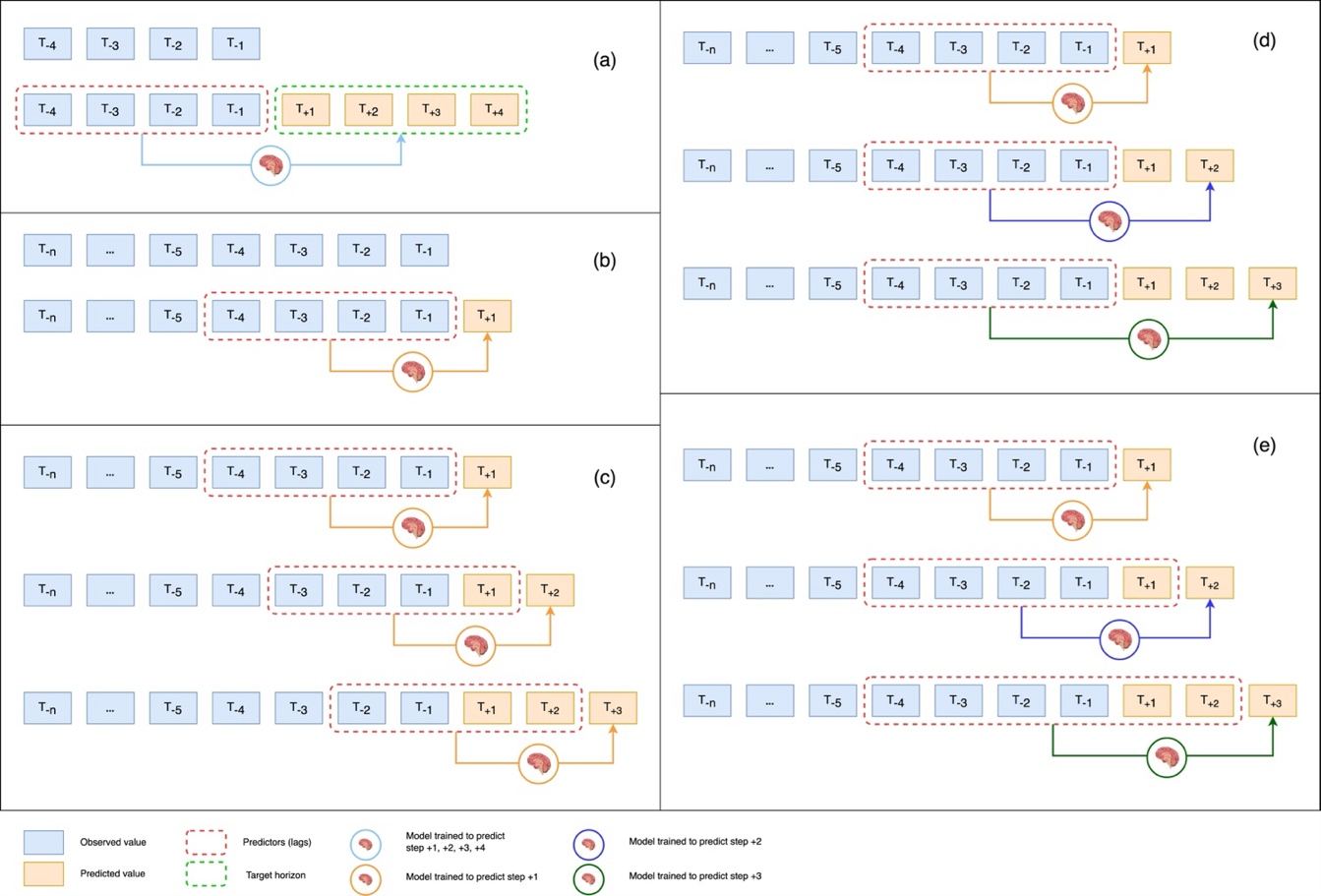
Figure 3. Illustration of time-steps in time series forecasting with (a) multiple output forecasting, (b) single-step forecasting, (c) recursive multi-step forecasting, (d) direct multi-step forecasting, and (e) direct recursive multi-step forecasting
- COMPONENTS IN TIME SERIES
Time series data consists of four key elements that are relevant to analyzing and predicting change over time [48]-[50]. One basic component is the trend, which is the long-term movement of the data. A trend captures the general direction of the data, whether it is moving up, down, or stable within a certain range over a period of time [48],[51]. Trends can be linear, which shows a smooth, steady increase or decrease, or nonlinear, which shows a more complex pattern of movement where the rate of change varies over time. Linear trends can occur in cases such as steady population growth, where there is a uniform increase each year. Nonlinear trends can be seen in technology adoption, where there is accelerated growth over time as more people accept the technology. It is important to understand the components of a trend because they provide the underlying overall movement of the data, helping analysts make long-term forecasts and sound decision strategies. The second component is seasonality, which consists of fluctuations that recur over a period of time [48],[52][53]. Seasonal variability usually occurs over a period of time, such as a day, week, month, or year and can be influenced by a variety of circumstances such as climate, periodic holidays, or other recurring phenomena. For example, many retailers see a spike in sales during the months leading up to Christmas as people shop for the holidays, or people may tend to buy more ice cream in the summer because the weather is warmer. Seasonal periods are always the same and are recurring events so they can predict when sales will go up or down which is fundamentally important for certain businesses in managing their inventory, expenses, marketing and headcount. Seasonal variations are clearly defined patterns that can be easily predicted. As a result, seasonal fluctuations are not random patterns and can be used for more precise short-term analysis. These patterns of events help businesses to accurately track when anticipating in the short term by identifying which events are predictable and are caused by time-driven factors.
The third component, cyclical variations, refers to periodic long-term changes over a defined time span [48],[54]. Unlike seasonal, cyclical variations take longer and are less certain to develop. They are primarily associated with larger business or economic cycles such as economic booms or recessions, which last for several years. Unlike seasonal patterns which can be accurately predicted based on their regular occurrence, cyclical fluctuations are more difficult to forecast due to the economy’s dependence on a variety of unpredictable factors. A good example is a company experiencing lower sales and profits during an economic downturn, but there is no set time or duration for these cycles. Nonetheless, these movements help businesses and economists gain new perspective on the specific region or market their industry is facing while considering the broader economy. While the last is irregular fluctuations or random fluctuations are random deviations as a result of unanticipated events that can occur outside of established trends, seasons, or cyclical changes [48],[50],[57]. These irregularities can come from sudden changes in the market, catastrophic events, technological shifts, or errors made when collecting data. Especially during time series analysis, this must be handled with great care because without proper handling, irregularities can mask existing trends or patterns and cause confusion when trying to draw important conclusions from the data. For example, the emergence of a new intense political challenge can cause a decline in confidence in the market leading to confusing stock movements that cannot be explained using seasonal or economic cycle indicators. The differences between these four components of time series data are shown in Figure 4.
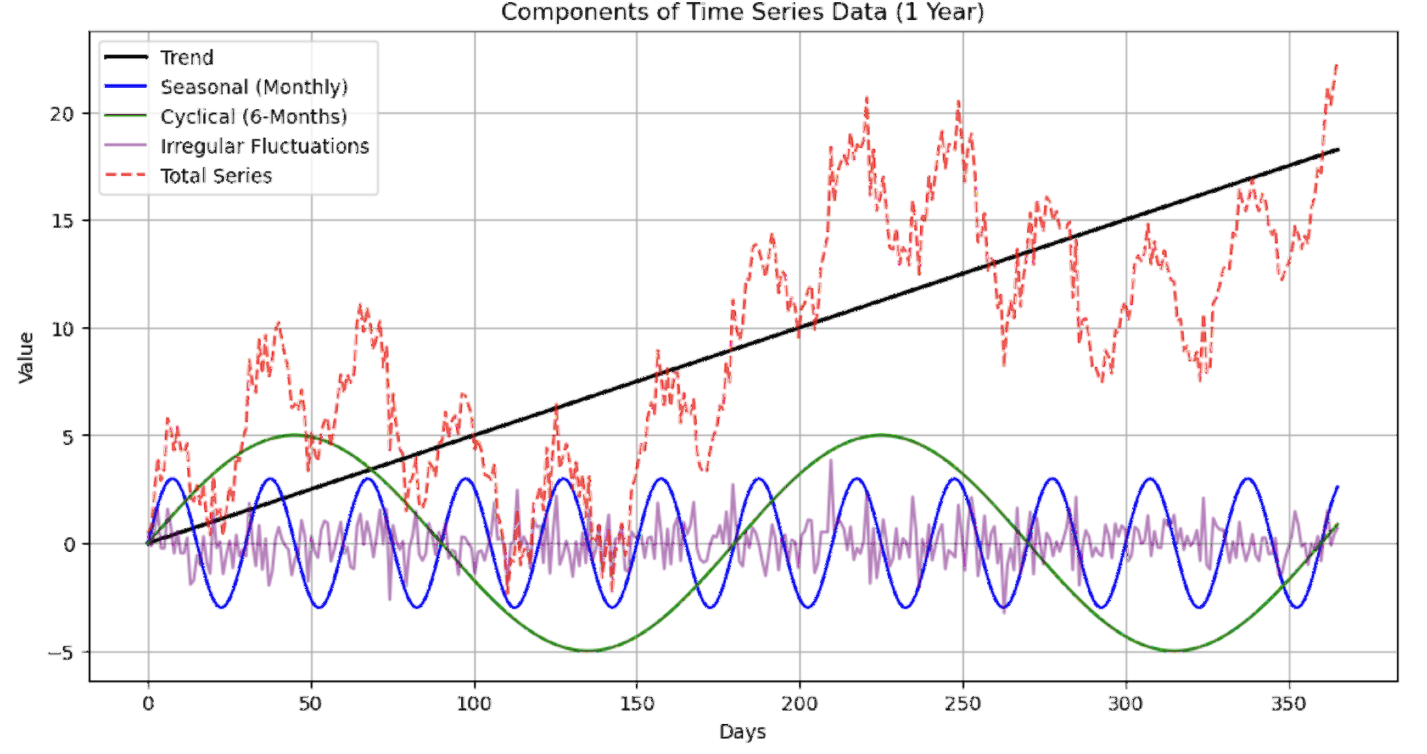
Figure 4. Comparison of time series data components within a year; Trend (black line): Slow but steady linear increase, Seasonal (blue line): Seasonal fluctuations that repeat every month. Cyclical (green line): Long-term cyclical pattern with a frequency of about six months, Irregular fluctuations (purple line): Random fluctuations that show erratic variations, Total Series (red dashed line): Sum of all components [55][56].
- DATA PREPROCESSING IN TIME SERIES FORECASTING
Data preprocessing is basically a systematic task that converts raw data into a machine-readable format for further analysis and modeling [58][59]. This task involves various steps related to data integrity, quality, and efficiency, among others. There is a comprehensive data preprocessing pipeline that improves model performance and ensures reliable model output. This process starts with Lineage/Provenance, which determines the origin, changes made to the data, and the lifecycle history of the data. For the sake of transparency, accountability, and reproducibility, this ensures that analysts and researchers can validate the source of information in a human-like manner. Knowing from where the data was taken and how it was changed helps in validating or ensuring the validity of downstream analysis. After that, there is Sampling which is the process of selecting a portion of a larger data set that is representative of the actual data [60]. When the data set is very large, full-scale processing becomes computationally expensive and time-consuming. By taking a portion of the data that is representative of this data set, we can ensure a balance between accuracy and efficiency without losing significant information. Depending on the structure and requirements of the dataset, different sampling methods can be adopted, such as stratified sampling, random sampling, or systematic sampling.
Once the samples are selected, move on to the Data Cleaning phase, where the information in the dataset is checked for inconsistencies, errors, and other forms of irregularities [61]-[63]. The first problem identified in this stage is called Noise which is defined as random deviations, irrelevant changes, or errors in the data that can distort the pattern and have a major impact on the accuracy of the model. Malfunctioning sensors, data transmission errors, or even some errors made by human input can cause noise. In order for the dataset to be reliable for analysis, noise needs to be removed. Another effective approach to data cleaning is to address Outliers which are defined as abnormal or exceptional values that fall outside the normal distribution range of the dataset. Caused by measurement errors or real anomalies, outliers do have an impact that needs to be investigated more closely. Outlier values can be handled by transforming them, removing them, or introducing some statistical countermeasures such as, “winsorization” or strong standardization.
Another major challenge associated with data cleaning is Missing Data which inevitably refers to data values that should be present but for some reason, are missing [64][65]. Missing data values can occur due to malfunctioning sensors, incomplete survey forms, data entry errors, or other technical errors. Assuming there are missing values in the data, some level of estimation (mean, median, or predictive) or deletion (either listwise or pairwise) can be applied to address them. The term filling missing values is often referred to as imputation techniques. Additionally, redundant records known as Duplicates that appear more than once in the dataset also need to be found and removed, otherwise the analysis will be flawed [66]. Such records can increase some counts in observations and skew certain statistics, which will be predicted inaccurately. Removing these ensures that all observations are reliable and every data point is useful to the predictive model.
After that, now that the data is clean and free from any inconsistencies, the next stage is Sensor/Data Fusion. During this phase, data from multiple sources or sensors are combined and integrated into a single source [67][68]. This ensures better completeness, consistency, and reliability of the data. When data is combined from multiple sources, errors are minimized and uncertainties are reduced, thus providing a more accurate picture of the phenomenon being investigated. For example, during air quality monitoring, data collected from multiple sensors located at different positions can be used to generate a more accurate pollution index. The data collected from these multiple sources is assumed to have gone through the data cleaning process, so that there is no more noise in the data that must be addressed in subsequent stages. This data fusion stage is carried out after data cleaning aims to ensure the quality and consistency of the data before merging, thereby preventing the propagation of errors into the larger dataset.
After having a comprehensive structured integrated dataset, the next step is Privacy Protection, which involves restricting sensitive or personal information from being accessed or violated by unauthorized personnel [69]. However, this stage is actually quite flexible because it can be done earlier by the research and analyst team. In today’s highly automated and data-driven world, privacy intrusion has emerged as a challenge and threat especially when dealing with personally identifiable information (PII) and sensitive data. Data that is supposed to be used for analysis such as personal information is protected through methods such as anonymization, differential privacy, and encryption. Privacy protection is especially important when dealing with medical, financial, or behavioral data of users. Once data privacy is well protected, the Windowing/Partitioning technique can be used to divide the dataset into smaller, semantically meaningful chunks. This technique is especially useful for dealing with time series data in analysis, as well as data that is processed in real-time. Windowing facilitates the structuring of data into segments for analysis, where each segment is treated individually to detect trends and patterns. Partitioning also helps in parallel processing, where different segments of the dataset are processed independently and the analyzed data is compiled for the final output. Similar to Privacy Protection, the Windowing stage is also flexible. This stage is not a mandatory stage, but an optional stage if needed in the analysis.
In addition, the next step that can be taken is Normalization. This is the process of correcting data that has been scaled differently to fit a common scale. This is especially important for machine learning models that differ in sensitivity to scale differences such as neural networks and gradient-based algorithms. With min-max scaling, Z-score normalization, and decimal scaling, no feature is allowed to dominate due to variations in magnitude. The normalization step is performed after windowing to prevent data leakage between window segments, ensure appropriate scales within each window, improve processing efficiency, and provide flexibility in choosing a normalization method. If normalization is performed first, the data scale can be affected by the entire dataset, causing mismatches between windows and potential data leakage, especially in time series analysis. By applying windowing first, each data segment can be normalized independently based on its characteristics, making the analysis results more accurate and efficient. However, this step may be adjusted as needed. The next step of normalization is debiasing which is the process of removing bias in the data set. Unbalanced data distribution, unfairness from history, or sample data can cause bias. These biases must be addressed to ensure that the model predictions are objective and unbiased.
Once the dataset is structured, cleaned, and normalized, feature engineering begins [70]. This is the step where new features and even modifications to certain features are done with the aim of improving the performance of the model. Feature engineering begins with Transformation, which is defined as changing the data into a form suitable for analysis. One of the processes that occurs during transformation is called Dimensionality Change, which means changing the number of features by making them more complex or simpler by removing unimportant features. Categorical bins can capture certain patterns and therefore Discretization makes it possible by converting continuous numbers to categorical data. Precision Change balances detail with computational needs, while numeric values are limited in scope. In Type Conversion, the values are formatted into machine learning capabilities such as integers, pointers, or floats, and used as basic machine learning data types.
Apart from transformation, another aspect of feature engineering is called Synthesis. This involves producing new features from existing features through mathematical functions, aggregations, or special manipulations. Feature synthesis allows the model to exploit hidden relationships within the data leading to improved model performance. After synthesis, redundant or irrelevant features are removed in Feature Reduction which improves computational efficiency and retains important information. In the final phase of feature reduction, Feature Extraction combines Expert Systems and knowledge-based systems, where in-depth data is obtained through Principal Component Analysis (PCA) or using autoencoders [71][72]. However, Feature Selection extracts the features that add the most value to the predictive power of the model [73], while ignoring the features that do not drive value. The final stage that can be performed in this preprocessing is Compression. This stage is a process that takes a dataset and reduces its size with respect to the goal of retaining as much value as possible. Dimensionality reduction, quantization, or encoding are all considered effective compression techniques that help optimize storage and computation, leading to faster and more efficient data processing. This is especially useful in the context of big data where it becomes essential to reduce the volume of the dataset while retaining important information for analysis. These methodical approaches ensure that the dataset will be clean, well-structured, and optimized for analysis leading to better model performance and reliable insights. Suggested sequence in the data preprocessing stage is shown in Figure 5.
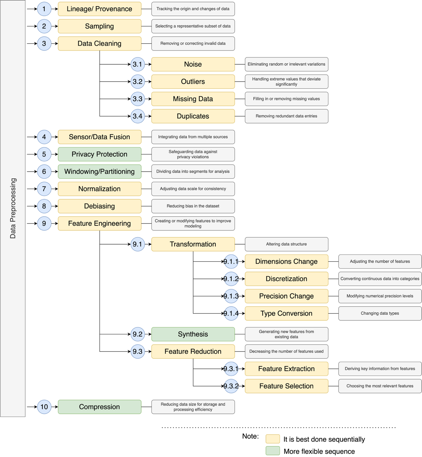
Figure 5. Data preprocessing in order to improve the quality of time series forecasting data [79] with recommendations that are best done sequentially (yellow) and flexible sequence (green)
- POPULAR METHOD FOR TIME SERIES FORECASTING
As explained in section: III. General Stages in Time Series Forecasting, that in general the methods in forecasting are divided into two parts, namely qualitative and quantitative methods. In the context of time series forecasting, it is included in quantitative methods along with causal methods, as shown in Figure 6. In time series forecasting, quantitative methods are used to predict future values based on previously recorded data in chronological order. One of the most well-known methods is ARIMA, which consists of three main components: Auto Regressive (AR), Moving Average (MA), and Integrated (I) [9],[74]. The AR component assesses how much the current value depends on past values in the data, while MA predicts errors that occurred in the previous period. The Integrated (I) component is responsible for making the data stationary by removing long-term trends or changes in the data [75]. ARIMA is suitable for data sets that do not show clear seasonal patterns, but for those that show seasonal patterns, SARIMA (Seasonal ARIMA) can be applied [76][77]. SARIMA adds a seasonal component to ARIMA to accommodate data that shows regular seasonal patterns. In addition, ARFIMA is used for data with long-term dependencies [78], meaning that values in the distant future are highly determined by values in the distant past.
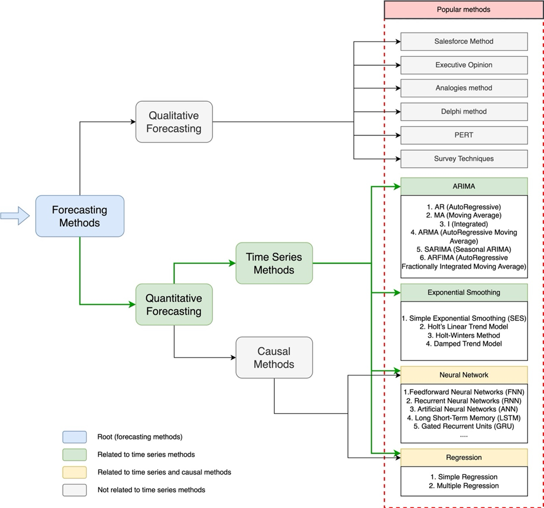
Figure 6. Time series methods are part of quantitative methods along with causal methods and several sub-parts of them
In addition to ARIMA, Exponential Smoothing is also widely used in time series forecasting, especially for data that does not have complex trends or seasonality [80][81]. Simple Exponential Smoothing (SES) gives more weight to the most recent data, making it suitable for stable data with no trends or seasonality [82]. However, for data with trends, the Holt Linear Trend Model can be applied because it considers not only the level of data, but also the trend in the data [83]. If the data also shows seasonal fluctuations, the Holt-Winters Method can be used, which adds a seasonal component to handle data that has a clear seasonal pattern [77]. There are also other variations such as the Damped Trend Model [84], which is useful for data that shows a gradually fading trend because it reduces the impact of the trend over time. In the case of more complex and non-linear time series data, Neural Networks offer a flexible approach, as well as the ability to handle relationships that are difficult to realize with traditional linear methods. Forward Neural Networks (FNNs) are relatively simple but can handle some forms of non-linear relationships between inputs and outputs [85]-[87]. However, for more sequential data, such as time series data, Recurrent Neural Networks (RNNs) are more effective because they can remember previous periods [88]-[90]. One of the most advanced variants of RNNs is Long Short-Term Memory (LSTM) [91], which was developed to address the vanishing gradient problem in RNNs and is able to retain information for longer periods of time, very useful for data with long-term dependencies [92]. Gated Recurrent Units (GRUs) [93][94] are a simpler but still effective and more efficient variant of RNNs that, unlike LSTMs, train faster.
While ARIMA and Neural Networks are considered the best models for time series forecasting, Regression techniques can also do the job easily, especially in cases where there is a causal relationship between time as a variable and other variable involved. Simple regression can be applied to a single independent variable affecting the dependent variable [95] in time series data, while multiple regression is applied when there are multiple independent variables affecting the dependent variable. Regression is usually not the dominant model in time series analysis, as it is more likely to be used for causal forecasting, but there are situations when regression can be used to model the relationship between relevant time series data. The choice of method in time series forecasting depends largely on the characteristics of the data at hand and the forecasting objectives to be achieved, and there is always a trade-off between ARIMA, Exponential Smoothing, Neural Networks, and Regression, each having its strengths in different contexts.
- VALIDATING TIME SERIES FORECASTING RESULTS
Based on what we have mentioned in section III. General Stages in Time Series Forecasting, to find out how reliable the model is, validation is needed which is an integral part of estimating the accuracy of the forecast. Validation of time series forecasting can be done in several steps and ways. Here we try to outline five parts, starting from data splitting, cross-validation [96], error metrics, residual analysis, to visualization, as shown in Figure 7. In this topic of time series forecasting, more attention needs to be paid to the time sequence and patterns contained in the data when generating and evaluating prediction models. The first step that must be taken is data splitting or dividing the data into two parts, training and testing [97]. In time series, data division must consider the time sequence, so that training data always precedes testing data. One method that can be used is out-of-sample validation, where the testing data is ensured to come from a different time period from which the training data was taken, so that the model is not tested using the same data as the training. On the other hand, rolling forecast origin is also often applied to time series, where the model is trained on data that is regularly updated with the latest data and is always tested on the latest data. This reflects the movement and changes in data over time. However, this certainly depends on the condition of the data used in forecasting. If the data is always updated, then this method can be a mainstay method. However, if not, then methods such as sequential validation can also be a strong alternative in splitting forecasting data while maintaining the time series sequence. Actually, this stage has been carried out before the data enters the training and forecasting stages. So, at this evaluation and validation stage, it is sufficient to use data that has been split previously. This step is one of the mandatory initial steps to ensure that the validation runs well because the data is appropriate.
Furthermore, to ensure that the model does not only memorize patterns in the training data, cross-validation is a solution that greatly encourages model generalization [98][99]. In the field of time series, expanding window is the most frequently used method. In this method, the size of the train data is incrementing, while the size of the test data is fixed. This allows the model to be from more data over time. Conversely, in a sliding window, the size of the training data is fixed and the data trained in it is the latest data. This approach allows testing how the model will adapt to changes in data patterns over time. After the model is trained and tested, the next step is to measure the model's performance using error metrics. In time series, popular forecast error evaluation metrics are Mean Absolute Error (MAE) [100][101], Root Mean Squared Error (RMSE) [95],[102], Mean Squared Error (MSE) [103]-[105], and Mean Absolute Percentage Error (MAPE). MAE and RMSE in this case are two metrics that help to understand the error considerations that occur in time series data, while MAPE is more appropriate to use if you want to measure how big the error is in percentage form. In addition, sMAPE is a more robust version of MAPE when the actual value is close to zero because the resulting evaluation is more balanced.
In addition, almost similar to error, residual analysis helps observers to see how well the model has adapted to the patterns in the data in the time series. The method that is often used is the autocorrelation function (ACF) [106], a feature that allows us to analyze time series. ACF helps to determine whether there is a correlation between residuals at different times. There is a significant correlation, it is an indication that the model still needs to capture more temporal patterns of its data behavior, such as trends or seasonality. This method is actually more suitable for regression methods if used at any time in the time series forecasting process. After the previous validation process is complete, visualization can be used, which is one of the most important methods in time series to help interpret and discuss the results of the model. Time series plots are the most frequently used graphs to directly see not only predictions, but also compare with actual values over time. In this way, it can create a visual interpretation of how well the data follows the trends and patterns in the data. In addition, error distribution plots, residual plots, and autocorrelation plots can also be used together with other plots to provide an overview of model errors and whether there are parts of the data that have not been learned well by the model.
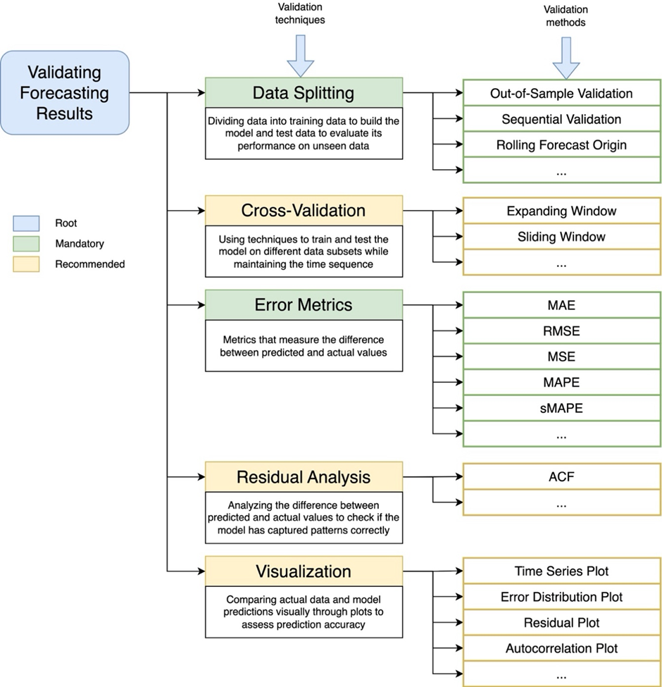
Figure 7. Validation techniques ranging from data splitting, cross-validation, error metrics, residual analysis, to visualization, along with several validation methods that are often used in time series forecasting. Green is marked as mandatory, while yellow is marked as a recommendation (optional)
- CONCLUSION
Predicting future events when based on historical data requires mastery of time series forecasting. There are many different components of time series forecasting, such as seasonality, trend analysis, cyclical variations, and irregular fluctuations, all of which are integral to understanding patterns in the data. Once the combination is identified and analyzed, the accuracy and reliability of the predictions will increase, making it more effective for businesses and researchers. Additionally, cleaning, structuring, and formatting the entire data to be analyzed must be handled during the preprocessing stage to ensure accuracy. Structuring and normalizing the data among other feature engineering techniques will enable the model to perform better, which will further result in higher accuracy in predicting outcomes. Depending on the type of data, whether linear, non-linear, seasonal, or non-seasonal, various approaches such as ARIMA, SARIMA, Exponential Smoothing, or even more sophisticated ones like Neural Networks can be used. The time series forecasting model is then validated to ensure its accuracy and reliability. Techniques such as cross-validation, error metrics, and residual analysis are essential for model evaluation and refinement. The fundamental study in this manuscript is expected to be the basis of understanding for time series forecasting researchers which will ultimately be very useful for institutions and organizations that need it in their business processes and others.
DECLARATION
Author Contribution
All authors contributed equally to the main contributor to this paper. All authors read and approved the final paper.
Funding
This research received no external funding.
Conflicts of Interest
The authors declare no conflict of interest.
REFERENCES
- S. S. W. Fatima and A. Rahimi, “A Review of Time-Series Forecasting Algorithms for Industrial Manufacturing Systems,” Machines, vol. 12, no. 6, p. 380, 2024, https://doi.org/10.3390/machines12060380.
- K. Choi, J. Yi, C. Park, and S. Yoon, “Deep Learning for Anomaly Detection in Time-Series Data: Review, Analysis, and Guidelines,” IEEE Access, vol. 9, pp. 120043–120065, 2021, https://doi.org/10.1109/ACCESS.2021.3107975.
- M. Pacella and G. Papadia, “Evaluation of deep learning with long short-term memory networks for time series forecasting in supply chain management,” Procedia CIRP, vol. 99, pp. 604–609, 2021, https://doi.org/10.1016/j.procir.2021.03.081.
- R. S. Mangrulkar and P. V. Chavan, “Time Series Analysis,” in Predictive Analytics with SAS and R, Berkeley, CA: Apress, pp. 121–165. 2025, https://doi.org/10.1007/979-8-8688-0905-7_5.
- D. Rifaldi et al., “Machine Learning 5.0 In-depth Analysis Trends in Classification,” Scientific Journal of Computer Science, vol. 1, no. 1, pp. 1–15, 2025, https://doi.org/10.64539/sjcs.v1i1.2025.18.
- J. F. Torres, D. Hadjout, A. Sebaa, F. Martínez-Álvarez, and A. Troncoso, “Deep Learning for Time Series Forecasting: A Survey,” Big Data, vol. 9, no. 1, pp. 3–21, 2021, https://doi.org/10.1089/big.2020.0159.
- A. M. Nakib and S. J. Haque, “Semi-Supervised Learning for Retinal Disease Detection: A BIOMISA Study,” Scientific Journal of Engineering Research, vol. 1, no. 2, pp. 43–53, 2025, https://doi.org/10.64539/sjer.v1i2.2025.14.
- M. Fahmi, A. Yudhana, Sunardi, A.-N. Sharkawy, and Furizal, “Classification for Waste Image in Convolutional Neural Network Using Morph-HSV Color Model,” Scientific Journal of Engineering Research, vol. 1, no. 1, pp. 18–25, 2025, https://doi.org/10.64539/sjer.v1i1.2025.12.
- M. K. Ho, H. Darman, and S. Musa, “Stock Price Prediction Using ARIMA, Neural Network and LSTM Models,” J Phys Conf Ser, vol. 1988, no. 1, p. 012041, 2021, https://doi.org/10.1088/1742-6596/1988/1/012041.
- M. Sakib, S. Mustajab, and M. Alam, “Ensemble deep learning techniques for time series analysis: a comprehensive review, applications, open issues, challenges, and future directions,” Cluster Comput, vol. 28, no. 1, p. 73, 2025, https://doi.org/10.1007/s10586-024-04684-0.
- Z. Liu, Z. Zhu, J. Gao, and C. Xu, “Forecast Methods for Time Series Data: A Survey,” IEEE Access, vol. 9, pp. 91896–91912, 2021, https://doi.org/10.1109/ACCESS.2021.3091162.
- E. Brophy, Z. Wang, Q. She, and T. Ward, “Generative Adversarial Networks in Time Series: A Systematic Literature Review,” ACM Comput Surv, vol. 55, no. 10, pp. 1–31, 2023, https://doi.org/10.1145/3559540.
- V. I. Kontopoulou, A. D. Panagopoulos, I. Kakkos, and G. K. Matsopoulos, “A Review of ARIMA vs. Machine Learning Approaches for Time Series Forecasting in Data Driven Networks,” Future Internet, vol. 15, no. 8, p. 255, 2023, https://doi.org/10.3390/fi15080255.
- S. F. Stefenon, L. O. Seman, V. C. Mariani, and L. dos S. Coelho, “Aggregating Prophet and Seasonal Trend Decomposition for Time Series Forecasting of Italian Electricity Spot Prices,” Energies (Basel), vol. 16, no. 3, p. 1371, 2023, https://doi.org/10.3390/en16031371.
- V. F. Silva, M. E. Silva, P. Ribeiro, and F. Silva, “Time series analysis via network science: Concepts and algorithms,” WIREs Data Mining and Knowledge Discovery, vol. 11, no. 3, 2021, https://doi.org/10.1002/widm.1404.
- C. Pino et al., “Intelligent Traction Inverter in Next Generation Electric Vehicles: The Health Monitoring of Silicon-Carbide Power Modules,” IEEE Transactions on Intelligent Vehicles, vol. 8, no. 12, pp. 4734–4753, 2023, https://doi.org/10.1109/TIV.2023.3294726.
- H. Lin et al., “Time series-based groundwater level forecasting using gated recurrent unit deep neural networks,” Engineering Applications of Computational Fluid Mechanics, vol. 16, no. 1, pp. 1655–1672, 2022, https://doi.org/10.1080/19942060.2022.2104928.
- V. Kotu and B. Deshpande, “Time Series Forecasting,” in Data Science, pp. 395–445, 2019, https://doi.org/10.1016/B978-0-12-814761-0.00012-5.
- Y. E. N. Nugraha, I. Ariawan, and W. A. Arifin, “Weather Forecast from Time Series Data Using LSTM Algorithm,” Jurnal Teknologi Informasi dan Komunikasi, vol. 14, no. 1, pp. 144–152, 2023, https://doi.org/10.51903/jtikp.v14i1.531.
- K. Benidis et al., “Deep Learning for Time Series Forecasting: Tutorial and Literature Survey,” ACM Comput Surv, vol. 55, no. 6, pp. 1–36, 2023, https://doi.org/10.1145/3533382.
- A. Tadjer, A. Hong, and R. B. Bratvold, “Machine learning based decline curve analysis for short-term oil production forecast,” Energy Exploration & Exploitation, vol. 39, no. 5, pp. 1747–1769, 2021, https://doi.org/10.1177/01445987211011784.
- N. Kashpruk, C. Piskor-Ignatowicz, and J. Baranowski, “Time Series Prediction in Industry 4.0: A Comprehensive Review and Prospects for Future Advancements,” Applied Sciences, vol. 13, no. 22, p. 12374, 2023, https://doi.org/10.3390/app132212374.
- B. Lim, S. Ö. Arık, N. Loeff, and T. Pfister, “Temporal Fusion Transformers for interpretable multi-horizon time series forecasting,” Int J Forecast, vol. 37, no. 4, pp. 1748–1764, 2021, https://doi.org/10.1016/j.ijforecast.2021.03.012.
- M. F. Azam and M. S. Younis, “Multi-Horizon Electricity Load and Price Forecasting Using an Interpretable Multi-Head Self-Attention and EEMD-Based Framework,” IEEE Access, vol. 9, pp. 85918–85932, 2021, https://doi.org/10.1109/ACCESS.2021.3086039.
- S. F. Ahamed, A. Vijayasankar, M. Thenmozhi, S. Rajendar, P. Bindu, and T. Subha Mastan Rao, “Machine learning models for forecasting and estimation of business operations,” The Journal of High Technology Management Research, vol. 34, no. 1, p. 100455, 2023, https://doi.org/10.1016/j.hitech.2023.100455.
- M. A. Pilin, “The past of predicting the future: A review of the multidisciplinary history of affective forecasting,” Hist Human Sci, vol. 34, no. 3–4, pp. 290–306, 2021, https://doi.org/10.1177/0952695120976330.
- A. Nandan Prasad, “Data Quality and Preprocessing,” in Introduction to Data Governance for Machine Learning Systems, pp. 109–223, 2024, https://doi.org/10.1007/979-8-8688-1023-7_3.
- M. Usmani, Z. A. Memon, A. Zulfiqar, and R. Qureshi, “Preptimize: Automation of Time Series Data Preprocessing and Forecasting,” Algorithms, vol. 17, no. 8, p. 332, 2024, https://doi.org/10.3390/a17080332.
- R. Hasanah et al., “Play Store Data Scrapping and Preprocessing done as Sentiment Analysis Material,” Indonesian Journal of Modern Science and Technology (IJMST), vol. 1, no. 1, pp. 16–21, 2025, https://doi.org/10.64021/ijmst.1.1.16-21.2025.
- A. R. N. Habibi et al., “Diabetes Mellitus Disease Analysis using Support Vector Machines and K-Nearest Neighbor Methods,” Indonesian Journal of Modern Science and Technology (IJMST), vol. 1, no. 1, pp. 22–27, 2025, https://doi.org/10.64021/ijmst.1.1.22-27.2025.
- R. F. N. Nurfalah, D. P. Hostiadi, and E. Triandini, “Performance Analysis of Prediction Methods on Tokyo Airbnb Data: A Comparative Study of Hyperparameter-Tuned XGBoost, ARIMA, and LSTM,” Jurnal Ilmiah Teknik Elektro Komputer dan Informatika, vol. 11, no. 2, pp. 184–193, 2025, https://doi.org/10.26555/jiteki.v11i2.30631.
- A. Ajiono, “Comparison of Three Time Series Forecasting Methods on Linear Regression, Exponential Smoothing and Weighted Moving Average,” IJIIS: International Journal of Informatics and Information Systems, vol. 6, no. 2, pp. 89–102, 2023, https://doi.org/10.47738/ijiis.v6i2.165.
- Md. T. Hossain, R. Afrin, and Mohd. A.-A. Biswas, “A Review on Attacks against Artificial Intelligence (AI) and Their Defence Image Recognition and Generation Machine Learning, Artificial Intelligence,” Control Systems and Optimization Letters, vol. 2, no. 1, pp. 52–59, 2024, https://doi.org/10.59247/csol.v2i1.73.
- M. Yunus, M. K. Biddinika, and A. Fadlil, “Comparison of Machine Learning Algorithms for Stunting Classification,” Scientific Journal of Engineering Research, vol. 1, no. 2, pp. 64–70, 2025, https://doi.org/10.64539/sjer.v1i2.2025.9.
- Md. M. U. Qureshi, A. B. Ahmed, A. Dulmini, M. M. H. Khan, and R. Rois, “Developing a seasonal-adjusted machine-learning-based hybrid time-series model to forecast heatwave warning,” Sci Rep, vol. 15, no. 1, p. 8699, 2025, https://doi.org/10.1038/s41598-025-93227-7.
- N. Maleki, O. Lundström, A. Musaddiq, J. Jeansson, T. Olsson, and F. Ahlgren, “Future energy insights: Time-series and deep learning models for city load forecasting,” Appl Energy, vol. 374, p. 124067, 2024, https://doi.org/10.1016/j.apenergy.2024.124067.
- M. Sahani, S. Choudhury, M. D. Siddique, T. Parida, P. K. Dash, and S. K. Panda, “Precise single step and multistep short-term photovoltaic parameters forecasting based on reduced deep convolutional stack autoencoder and minimum variance multikernel random vector functional network,” Eng Appl Artif Intell, vol. 136, p. 108935, 2024, https://doi.org/10.1016/j.engappai.2024.108935.
- M. Omar, F. Yakub, S. S. Abdullah, M. S. A. Rahim, A. H. Zuhairi, and N. Govindan, “One-step vs horizon-step training strategies for multi-step traffic flow forecasting with direct particle swarm optimization grid search support vector regression and long short-term memory,” Expert Syst Appl, vol. 252, p. 124154, 2024, https://doi.org/10.1016/j.eswa.2024.124154.
- R. Chandra, S. Goyal, and R. Gupta, “Evaluation of Deep Learning Models for Multi-Step Ahead Time Series Prediction,” IEEE Access, vol. 9, pp. 83105–83123, 2021, https://doi.org/10.1109/ACCESS.2021.3085085.
- S. Suradhaniwar, S. Kar, S. S. Durbha, and A. Jagarlapudi, “Time Series Forecasting of Univariate Agrometeorological Data: A Comparative Performance Evaluation via One-Step and Multi-Step Ahead Forecasting Strategies,” Sensors, vol. 21, no. 7, p. 2430, 2021, https://doi.org/10.3390/s21072430.
- X. He, S. Shi, X. Geng, J. Yu, and L. Xu, “Multi-step forecasting of multivariate time series using multi-attention collaborative network,” Expert Syst Appl, vol. 211, p. 118516, 2023, https://doi.org/10.1016/j.eswa.2022.118516.
- J. Rebollo, S. Khater, and W. J. Coupe, “A Recursive Multi-step Machine Learning Approach for Airport Configuration Prediction,” in AIAA AVIATION 2021 FORUM, p. 2406, 2021, https://doi.org/10.2514/6.2021-2406.
- J. Gómez-Gómez, E. Gutiérrez de Ravé, and F. J. Jiménez-Hornero, “Assessment of Deep Neural Network Models for Direct and Recursive Multi-Step Prediction of PM10 in Southern Spain,” Forecasting, vol. 7, no. 1, p. 6, 2025, https://doi.org/10.3390/forecast7010006.
- E. Dolgintseva, H. Wu, O. Petrosian, A. Zhadan, A. Allakhverdyan, and A. Martemyanov, “Comparison of multi-step forecasting methods for renewable energy,” Energy Systems, pp. 1-32, 2024, https://doi.org/10.1007/s12667-024-00656-w.
- F. Nie, X. Li, P. Xu, X. Tian, and H. Zhou, “Short-term Load Forecasting Based on Text Encoding of External Variables,” TechRxiv, 2025, https://doi.org/10.36227/techrxiv.174585614.46388244/v1.
- E. Noa-Yarasca, J. M. Osorio Leyton, and J. P. Angerer, “Extending Multi-Output Methods for Long-Term Aboveground Biomass Time Series Forecasting Using Convolutional Neural Networks,” Mach Learn Knowl Extr, vol. 6, no. 3, pp. 1633–1652, 2024, https://doi.org/10.3390/make6030079.
- P. Nikolaidis, “Smart Grid Forecasting with MIMO Models: A Comparative Study of Machine Learning Techniques for Day-Ahead Residual Load Prediction,” Energies (Basel), vol. 17, no. 20, p. 5219, 2024, https://doi.org/10.3390/en17205219.
- K. Kyo, H. Noda, and F. Fang, “An integrated approach for decomposing time series data into trend, cycle and seasonal components,” Math Comput Model Dyn Syst, vol. 30, no. 1, pp. 792–813, 2024, https://doi.org/10.1080/13873954.2024.2416631.
- P. Das and S. Barman, “Perspective Chapter: An Overview of Time Series Decomposition and Its Applications,” in Applied and Theoretical Econometrics and Financial Crises [Working Title], 2025, https://doi.org/10.5772/intechopen.1009268.
- N. Entezari and J. A. Fuinhas, “Measuring wholesale electricity price risk from climate change: Evidence from Portugal,” Util Policy, vol. 91, p. 101837, 2024, https://doi.org/10.1016/j.jup.2024.101837.
- M. Yang, Y. Jiang, C. Xu, B. Wang, Z. Wang, and X. Su, “Day-ahead wind farm cluster power prediction based on trend categorization and spatial information integration model,” Appl Energy, vol. 388, p. 125580, 2025, https://doi.org/10.1016/j.apenergy.2025.125580.
- J. Li, Z.-L. Li, H. Wu, and N. You, “Trend, seasonality, and abrupt change detection method for land surface temperature time-series analysis: Evaluation and improvement,” Remote Sens Environ, vol. 280, p. 113222, 2022, https://doi.org/10.1016/j.rse.2022.113222.
- Y. Ensafi, S. H. Amin, G. Zhang, and B. Shah, “Time-series forecasting of seasonal items sales using machine learning – A comparative analysis,” International Journal of Information Management Data Insights, vol. 2, no. 1, p. 100058, 2022, https://doi.org/10.1016/j.jjimei.2022.100058.
- L. Ma, Y. Kojima, K. Nomoto, M. Hasegawa, and S. Hirobayashi, “Analysis of Cyclical Fluctuations in the Chinese Stock Market Using Non-Harmonic Analysis: Market Responses to Major Economic Events,” in 2024 10th International Conference on Systems and Informatics (ICSAI), IEEE, pp. 1–6, 2024, https://doi.org/10.1109/ICSAI65059.2024.10893771.
- G. Ciaburro and G. Iannace, “Machine Learning-Based Algorithms to Knowledge Extraction from Time Series Data: A Review,” Data (Basel), vol. 6, no. 6, p. 55, 2021, https://doi.org/10.3390/data6060055.
- J. Kim, H. Kim, H. Kim, D. Lee, and S. Yoon, “A comprehensive survey of deep learning for time series forecasting: architectural diversity and open challenges,” Artif Intell Rev, vol. 58, no. 7, p. 216, 2025, https://doi.org/10.1007/s10462-025-11223-9.
- F. Sun, X. Meng, Y. Zhang, Y. Wang, H. Jiang, and P. Liu, “Agricultural Product Price Forecasting Methods: A Review,” Agriculture, vol. 13, no. 9, p. 1671, 2023, https://doi.org/10.3390/agriculture13091671.
- P. Martins, F. Cardoso, P. Váz, J. Silva, and M. Abbasi, “Performance and Scalability of Data Cleaning and Preprocessing Tools: A Benchmark on Large Real-World Datasets,” Data (Basel), vol. 10, no. 5, p. 68, 2025, https://doi.org/10.3390/data10050068.
- A. Ebrahimi, H. V. Sefat, and J. Amani Rad, “Basics of machine learning,” in Dimensionality Reduction in Machine Learning, pp. 3–38, 2025, https://doi.org/10.1016/B978-0-44-332818-3.00009-5.
- A. Omair, “Sample size estimation and sampling techniques for selecting a representative sample,” Journal of Health Specialties, vol. 2, no. 4, p. 142, 2014, https://doi.org/10.4103/1658-600X.142783.
- M. Hosseinzadeh et al., “Data cleansing mechanisms and approaches for big data analytics: a systematic study,” J Ambient Intell Humaniz Comput, vol. 14, no. 1, pp. 99–111, 2023, https://doi.org/10.1007/s12652-021-03590-2.
- P. Li, X. Rao, J. Blase, Y. Zhang, X. Chu, and C. Zhang, “CleanML: A Study for Evaluating the Impact of Data Cleaning on ML Classification Tasks,” in 2021 IEEE 37th International Conference on Data Engineering (ICDE), pp. 13–24, 2021, https://doi.org/10.1109/ICDE51399.2021.00009.
- I. F. Ilyas and T. Rekatsinas, “Machine Learning and Data Cleaning: Which Serves the Other?,” Journal of Data and Information Quality, vol. 14, no. 3, pp. 1–11, 2022, https://doi.org/10.1145/3506712.
- G. J. Mellenbergh, “Missing Data,” in Counteracting Methodological Errors in Behavioral Research, pp. 275–292, 2019, https://doi.org/10.1007/978-3-030-12272-0_16.
- H. M. Kang, F. Yusof, and I. Mohamad, “Imputation of Missing Data with Different Missingness Mechanism,” J Teknol, vol. 57, no. 1, 2012, https://doi.org/10.11113/jt.v57.1523.
- A. Maulana et al., “Classification of Stunting inToddlers using Naive Bayes Method and Decision Tree,” Indonesian Journal of Modern Science and Technology (IJMST), vol. 1, no. 1, pp. 28–33, 2025, https://doi.org/10.64021/ijmst.1.1.28-33.2025.
- B. Erfianto and A. Rahmatsyah, “Application of ARIMA Kalman Filter with Multi-Sensor Data Fusion Fuzzy Logic to Improve Indoor Air Quality Index Estimation,” JOIV : International Journal on Informatics Visualization, vol. 6, no. 4, p. 771, 2022, https://doi.org/10.30630/joiv.6.4.889.
- W. Jing et al., “Application of Multiple-Source Data Fusion for the Discrimination of Two Botanical Origins of Magnolia Officinalis Cortex Based on E-Nose Measurements, E-Tongue Measurements, and Chemical Analysis,” Molecules, vol. 27, no. 12, p. 3892, 2022, https://doi.org/10.3390/molecules27123892.
- E. Di Minin, C. Fink, A. Hausmann, J. Kremer, and R. Kulkarni, “How to address data privacy concerns when using social media data in conservation science,” Conservation Biology, vol. 35, no. 2, pp. 437–446, 2021, https://doi.org/10.1111/cobi.13708.
- T. Verdonck, B. Baesens, M. Óskarsdóttir, and S. vanden Broucke, “Special issue on feature engineering editorial,” Mach Learn, vol. 113, no. 7, pp. 3917–3928, 2024, https://doi.org/10.1007/s10994-021-06042-2.
- A.-M. Tăuţan, A. C. Rossi, R. de Francisco, and B. Ionescu, “Dimensionality reduction for EEG-based sleep stage detection: comparison of autoencoders, principal component analysis and factor analysis,” Biomedical Engineering / Biomedizinische Technik, vol. 66, no. 2, pp. 125–136, 2021, https://doi.org/10.1515/bmt-2020-0139.
- Z. Salekshahrezaee, J. L. Leevy, and T. M. Khoshgoftaar, “Feature Extraction for Class Imbalance Using a Convolutional Autoencoder and Data Sampling,” in 2021 IEEE 33rd International Conference on Tools with Artificial Intelligence (ICTAI), pp. 217–223, 2021, https://doi.org/10.1109/ICTAI52525.2021.00037.
- N. Pudjihartono, T. Fadason, A. W. Kempa-Liehr, and J. M. O’Sullivan, “A Review of Feature Selection Methods for Machine Learning-Based Disease Risk Prediction,” Frontiers in Bioinformatics, vol. 2, 2022, https://doi.org/10.3389/fbinf.2022.927312.
- Y. Ning, H. Kazemi, and P. Tahmasebi, “A comparative machine learning study for time series oil production forecasting: ARIMA, LSTM, and Prophet,” Comput Geosci, vol. 164, p. 105126, 2022, https://doi.org/10.1016/j.cageo.2022.105126.
- S. Siami-Namini, N. Tavakoli, and A. Siami Namin, “A Comparison of ARIMA and LSTM in Forecasting Time Series,” in 2018 17th IEEE International Conference on Machine Learning and Applications (ICMLA), pp. 1394–1401, 2018, https://doi.org/10.1109/ICMLA.2018.00227.
- A. Parasyris, G. Alexandrakis, G. V. Kozyrakis, K. Spanoudaki, and N. A. Kampanis, “Predicting Meteorological Variables on Local Level with SARIMA, LSTM and Hybrid Techniques,” Atmosphere (Basel), vol. 13, no. 6, p. 878, 2022, https://doi.org/10.3390/atmos13060878.
- G. R. Alonso Brito, A. Rivero Villaverde, A. Lau Quan, and M. E. Ruíz Pérez, “Comparison between SARIMA and Holt–Winters models for forecasting monthly streamflow in the western region of Cuba,” SN Appl Sci, vol. 3, no. 6, p. 671, 2021, https://doi.org/10.1007/s42452-021-04667-5.
- A. N. A. Mahmad Azan, N. F. A. Mohd Zulkifly Mototo, and P. J. W. Mah, “The Comparison between ARIMA and ARFIMA Model to Forecast Kijang Emas (Gold) Prices in Malaysia using MAE, RMSE and MAPE,” Journal of Computing Research and Innovation, vol. 6, no. 3, pp. 22–33, 2021, https://doi.org/10.24191/jcrinn.v6i3.225.
- A. Tawakuli, B. Havers, V. Gulisano, D. Kaiser, and T. Engel, “Survey:Time-series data preprocessing: A survey and an empirical analysis,” Journal of Engineering Research, vol. 13, no. 2, pp. 674-711, 2024, https://doi.org/10.1016/j.jer.2024.02.018.
- C. Wiedyaningsih, E. Yuniarti, and N. P. V. Ginanti Putri, “Comparison of Forecasting Drug Needs Using Time Series Methods in Healthcare Facilities: A Systematic Review,” Jurnal Farmasi Sains dan Praktis, pp. 156–165, 2024, https://doi.org/10.31603/pharmacy.v10i2.11145.
- M. M. Abdullah, “Using the Single-Exponential-Smoothing Time Series Model under the Additive Holt-Winters Algorithm with Decomposition and Residual Analysis to Forecast the Reinsurance-Revenues Dataset,” Pakistan Journal of Statistics and Operation Research, pp. 311–340, 2024, https://doi.org/10.18187/pjsor.v20i2.4409.
- M. H. Abdelati and Hilal A. Abdelwali, “Optimizing Simple Exponential Smoothing for Time Series Forecasting in Supply Chain Management,” Indonesian Journal of Innovation and Applied Sciences (IJIAS), vol. 4, no. 3, pp. 247–256, 2024, https://doi.org/10.47540/ijias.v4i3.1591.
- A. Kumar and B. Meena, “A comparative analysis of the Holt and ARIMA models for predicting the future total fertility rate in India,” Life Cycle Reliability and Safety Engineering, vol. 14, no. 1, pp. 117–126, 2025, https://doi.org/10.1007/s41872-024-00287-1.
- A. Corberán-Vallet, E. Vercher, J. V. Segura, and J. D. Bermúdez, “A new approach to portfolio selection based on forecasting,” Expert Syst Appl, vol. 215, p. 119370, 2023, https://doi.org/10.1016/j.eswa.2022.119370.
- B. Warsito, R. Santoso, Suparti, and H. Yasin, “Cascade Forward Neural Network for Time Series Prediction,” J Phys Conf Ser, vol. 1025, p. 012097, 2018, https://doi.org/10.1088/1742-6596/1025/1/012097.
- Q. A. Al-Haija and N. A. Jebril, “Systemic framework of time-series prediction via feed-forward neural networks,” IET Conference Proceedings, vol. 2020, no. 6, pp. 583–588, 2021, https://doi.org/10.1049/icp.2021.0971.
- A. N. Sharkawy, “Forward and inverse kinematics solution of a robotic manipulator using a multilayer feedforward neural network,” Journal of Mechanical and Energy Engineering, vol. 6, no. 2, 2022, https://doi.org/10.30464/jmee.00300.
- D. I. Af’idah, Dairoh, and S. F. Handayani, “Comparative Analysis of Deep Learning Models for Retrieval-Based Tourism Information Chatbots,” Jurnal Ilmiah Teknik Elektro Komputer dan Informatika, vol. 11, no. 1, pp. 53–67, 2025, https://doi.org/10.26555/jiteki.v11i1.30373.
- I. Indriani and Y. Syukriyah, “The Use of Attention-RNN and Dense Layer Combinations and The Performance Metrics Achieved in Palm Vein Recognition,” Jurnal Ilmiah Teknik Elektro Komputer dan Informatika, vol. 11, no. 1, pp. 12–26, 2025, https://doi.org/10.26555/jiteki.v11i1.30517.
- I. Hossain, M. M. Islam, and Md. H. H. Martin, “Potential Applications and Limitations of Artificial Intelligence in Remote Sensing Data Interpretation: A Case Study,” Control Systems and Optimization Letters, vol. 2, no. 3, pp. 295–302, 2024, https://doi.org/10.59247/csol.v2i3.128.
- Poningsih, A. P. Windarto, and P. Alkhairi, “Reducing Overfitting in Neural Networks for Text Classification Using Kaggle’s IMDB Movie Reviews Dataset,” Jurnal Ilmiah Teknik Elektro Komputer dan Informatika, vol. 10, no. 3, pp. 534–543, 2024, https://doi.org/10.26555/jiteki.v10i3.29509.
- V. Monita, S. Raniprima, and N. Cahyadi, “Comparative Analysis of Daily and Weekly Heavy Rain Prediction Using LSTM and Cloud Data,” Jurnal Ilmiah Teknik Elektro Komputer dan Informatika, vol. 10, no. 4, pp. 833–842, 2024, https://doi.org/10.26555/jiteki.v10i4.30374.
- W. Riyadi and Jasmir, “Comparative Analysis of Optimizer Effectiveness in GRU and CNN-GRU Models for Airport Traffic Prediction,” Jurnal Ilmiah Teknik Elektro Komputer dan Informatika, vol. 10, no. 3, pp. 580–593, 2024, https://doi.org/10.26555/jiteki.v10i3.29659.
- H. Subair, R. P. Selvi, R. Vasanthi, S. Kokilavani, and V. Karthick, “Minimum Temperature Forecasting Using Gated Recurrent Unit,” International Journal of Environment and Climate Change, vol. 13, no. 9, pp. 2681–2688, 2023, https://doi.org/10.9734/ijecc/2023/v13i92499.
- A. B. Fawait, S. Rahmah, A. D. S. da Costa, N. Insyroh, and A. A. Firdaus, “Implementation of Data Mining Using Simple Linear Regression Algorithm to Predict Export Values,” Scientific Journal of Engineering Research, vol. 1, no. 1, pp. 26–32, 2025, https://doi.org/10.64539/sjer.v1i1.2025.11.
- C. D. Nariyana, M. Idhom, and Trimono, “Prediction of Purchase Volume Coffee Shops in Surabaya Using Catboost with Leave-One-Out Cross Validation,” Jurnal Ilmiah Teknik Elektro Komputer dan Informatika, vol. 11, no. 1, pp. 124–138, 2025, https://doi.org/10.26555/jiteki.v11i1.30610.
- M. Abidin et al., “Classification of Heart (Cardiovascular) Disease using the SVM Method,” Indonesian Journal of Modern Science and Technology (IJMST), vol. 1, no. 1, pp. 9–15, 2025, https://doi.org/10.64021/ijmst.1.1.9-15.2025.
- A. Abdul Aziz, M. Yusoff, W. F. W. Yaacob, and Z. Mustaffa, “Repeated time-series cross-validation: A new method to improved COVID-19 forecast accuracy in Malaysia,” MethodsX, vol. 13, p. 103013, 2024, https://doi.org/10.1016/j.mex.2024.103013.
- A. Maslan and A. Hamid, “Malware Classification and Detection using Variations of Machine Learning Algorithm Models,” Jurnal Ilmiah Teknik Elektro Komputer dan Informatika, vol. 11, no. 1, pp. 27–41, 2025, https://doi.org/10.26555/jiteki.v11i1.30477.
- M. M. Islam, Mst. T. Akter, H. M. Tahrim, N. S. Elme, and Md. Y. A. Khan, “A Review on Employing Weather Forecasts for Microgrids to Predict Solar Energy Generation with IoT and Artificial Neural Networks,” Control Systems and Optimization Letters, vol. 2, no. 2, pp. 184–190, 2024, https://doi.org/10.59247/csol.v2i2.108.
- D. S. K. Karunasingha, “Root mean square error or mean absolute error? Use their ratio as well,” Inf Sci (N Y), vol. 585, pp. 609–629, 2022, https://doi.org/10.1016/j.ins.2021.11.036.
- M. J. Kobra, M. O. Rahman, and A. M. Nakib, “A Novel Hybrid Framework for Noise Estimation in High-Tex-ture Images using Markov, MLE, and CNN Approaches,” Scientific Journal of Engineering Research, vol. 1, no. 2, pp. 54–63, 2025, https://doi.org/10.64539/sjer.v1i2.2025.25.
- F. Furizal, S. S. Mawarni, S. A. Akbar, A. Yudhana, and M. Kusno, “Analysis of the Influence of Number of Segments on Similarity Level in Wound Image Segmentation Using K-Means Clustering Algorithm,” Control Systems and Optimization Letters, vol. 1, no. 3, pp. 132–138, 2023, https://doi.org/10.59247/csol.v1i3.33.
- N. P. E. P. A. Adriani, R. R. Huizen, and D. Hermawan, “A Machine Learning-Based Approach for Retail Demand Forecasting: The Impact of Spending Score and Algorithm Optimization,” Jurnal Ilmiah Teknik Elektro Komputer dan Informatika, vol. 11, no. 2, pp. 169–183, 2025, https://doi.org/10.26555/jiteki.v11i2.30630.
- M. J. Kobra, A. M. Nakib, P. Mweetwa, and M. O. Rahman, “Effectiveness of Fourier, Wiener, Bilateral, and CLAHE Denoising Methods for CT Scan Image Noise Reduction,” Scientific Journal of Engineering Research, vol. 1, no. 3, pp. 96–108, 2025, https://doi.org/10.64539/sjer.v1i3.2025.27.
- J. F. Mgaya, “Application of ARIMA models in forecasting livestock products consumption in Tanzania,” Cogent Food Agric, vol. 5, no. 1, p. 1607430, 2019, https://doi.org/10.1080/23311932.2019.1607430.
AUTHOR BIOGRAPHY

| Furizal is a technology professional and researcher with a strong focus in intelligent systems and software development. Born in Riau, Indonesia, in 1999, he earned his Bachelor's degree in Informatics Engineering from Universitas Islam Riau in 2022, and completed his Master's degree in Informatics at Universitas Ahmad Dahlan in 2023. He began his professional career in 2021 as an IT Programmer at the Faculty of Engineering, Universitas Islam Riau. In 2024, he joined Bank Syariah Indonesia as an IT Programmer. Since 2025, he has served as the Director of Futuristech (PT. Teknologi Futuristik Indonesia), a company dedicated to developing cutting-edge technology solutions. His research interests include Deep Learning, Machine Learning, Artificial Intelligence, Fuzzy Logic, Control Systems, and the Internet of Things (IoT). E-mail: furizal.id@gmail.com |
|
|

| Alfian Ma’arif (Member, IEEE) was born in Klaten, Central Java, Indonesia, in 1991. He received the bachelor’s degree from the Department of Electrical Engineering, Universitas Islam Indonesia, in 2014, and the master’s degree from the Department of Electrical Engineering, Universitas Gadjah Mada, in 2017. From 2017 to 2018, he was a Lecturer with the Department of Electrical Engineering Education, Universitas Negeri Yogyakarta. Since 2018, he has been a Lecturer with the Department of Electrical Engineering, Universitas Ahmad Dahlan. He is currently an Assistant Professor, since 2020. His research interest includes control systems. He is a member of IAENG and ASCEE. He is the Editor in Chief of International Journal of Robotics and Control Systems and the Managing Editor of the Journal of Robotics and Control (JRC). E-mail: alfianmaarif@ee.uad.ac.id |
|
|

| Kariyamin earned a Bachelor's degree in Informatics Engineering from the Faculty of Computer Science, Universitas Muslim Indonesia, Makassar City, South Sulawesi, Indonesia in 2018. He then earned a Master's degree in Management at the Postgraduate Program of Universitas Muslim Indonesia, Makassar City, South Sulawesi, Indonesia in 2020. In 2024, he again earned a Master's degree in Informatics at the Postgraduate Program of Universitas Ahmad Dahlan, Yogyakarta, Indonesia. Since 2024, he has served as a permanent lecturer in the Information Technology Study Program, Institut Teknologi dan Bisnis Muhammadiyah Wakatobi. E-mail: karyaminyamin28@gmail.com |
|
|

| Asno Azzawagama Firdaus is a lecturer at Qamarul Huda University Badaruddin Bagu in the computer science study program. He took master's degree in Informatics at Ahmad Dahlan University, Indonesia and bachelor's degree in Informatics Engineering at Mataram University, Indonesia. He has a research focus on Artificial Intelligence, especially on NLP, Machine Learning, Data Analysis to Data Mining. E-mail: asnofirdaus@gmail.com |
|
|

| Setiawan Ardi Wijaya serves as a Lecturer in the Information Systems Study Program at the Faculty of Computer Science, Universitas Muhammadiyah Riau. He earned a Bachelor's degree in computer science from Universitas Muhammadiyah Purwokerto (2020) and a Master's degree in Informatics from the Faculty of Industrial Technology, Universitas Ahmad Dahlan (2022). His research interests include data analysis, computer science, computer vision, digital image processing and information systems. Email: setiawanardiwijaya@umri.ac.id |
|
|

| Arman Mohammad Nakib has been in teaching profession since 2015. He is doing PhD in East China Normal University, Shanghai, China and completed his master's in Artificial Intelligence and bachelor in Electrical and Electronic Engineering. His research focus on OCT Imaging, Medical Image Processing, Machine & Deep Learning, Computer Vision, Robotics, Multi-Sensor Data Processing, Internet of Things, Automation. Email: armannakib35@gmail.com |
|
|

| Ariska Fitriyana Ningrum serves as a Lecturer in the Data Science Program at the College of Fakultas Sains dan Teknologi Pertanian Universitas Muhammadiyah Semarang. She holds a Bachelor's degree in Statistik from Universitas Muhammadiyah Semarang (2020) and a Master's degree in statistik from Institut Teknologi Sepuluh Nopember, Surabaya (2023). Her research interests span multivariate time series, sentiment analyst, visual analytics, dan text mining. E-mail: ariskafitriyana@unimus.ac.id |
Furizal (Understanding Time Series Forecasting: A Fundamental Study)