ISSN: 2685-9572 Buletin Ilmiah Sarjana Teknik Elektro
Vol. 7, No. 3, September 2025, pp. 270-295
Comparative Performance Analysis of LQR Based PSO and Fuzzy Logic Control for Active Car Suspension
Ahmed J. Abougarair 1, Mohamed Aburakhis 2, Mohsen Bakouri 3, Alfian Ma’arif 4
1 Department of Electrical and Electronics Engineering, University of Tripoli, Tripoli, Libya
2 Electrical and Computer Engineering Department, Valparaiso University, Valparaiso, USA
3 Department of Medical Equipment Technology, Majmaah University, Majmaah City 11952, KSA
4 Department of Electrical Engineering, Universitas Ahmad Dahlan, Yogyakarta, Indonesia
ARTICLE INFORMATION |
| ABSTRACT |
Article History: Received 12 April 2025 Revised 03 June 2025 Accepted 09 July 2025 |
| 
This study proposes a diffrent control strategy for active car suspension systems, comparing the performance of Proportional-Integral-Derivative (PID), Linear Quadratic Regulator (LQR), and fuzzy PD controller in optimizing ride comfort and handling. These methods were selected for their complementary strengths: PID for simplicity and industrial adoption, LQR for optimality in handling trade-offs between ride comfort and suspension travel, and fuzzy PD for adaptability to nonlinearities and road disturbances. A 4-DOF quarter-car model is employed to simulate vehicle dynamics, with road disturbances modeled as step and sinusoidal inputs. The PID controller is tuned using built-in tools such as the PID tuner app, while the LQR’s weighting matrices (Q and R) were optimized offline using PSO. The optimized weights were then substituted into the algebraic Riccati equation to derive the final feedback control gains, ensuring optimal performance while adhering to classical LQR theory. For the fuzzy PD controller, membership functions and rule bases are designed to adaptively adjust gains under varying road conditions. Simulation results demonstrate that the PSO-tuned LQR and fuzzy PD controllers outperform conventional PID by reducing body vertical displacement by 61% and 23%, respectively, and overshoot by 75% (fuzzy PD) and 60.2% (LQR) under step excitation. The LQR controller based PSO also shows superior adaptability to stochastic road inputs and minimizing the control signal by 83.3% compared to PID. By integrating PSO-based LQR gain optimization and adaptive fuzzy logic, this work advances active suspension control, offering a quantifiably superior alternative to classical approaches. This study contributes to the technological development of the automotive world in order to provide comfort and safety for the passenger under different conditions, which contributes to the design of more comfortable vehicles with better performance in the future. |
Keywords: LQR; Fuzzy PD; PID; PSO; Suspension System |
Corresponding Author: Ahmed J. Abougarair, Department of Electrical and Electronics Engineering, University of Tripoli, Tripoli, Libya. Email: a.abougarair@uot.edu.ly |
This work is open access under a Creative Commons Attribution-Share Alike 4.0 
|
Document Citation: A. J. Abougarair, M. Aburakhis, M. Bakouri, and A. Ma’arif, “Comparative Performance Analysis of LQR Based PSO and Fuzzy Logic Control for Active Car Suspension,” Buletin Ilmiah Sarjana Teknik Elektro, vol. 7, no. 3, pp. 270-295, 2025, DOI: 10.12928/biste.v7i3.13237. |
- INTRODUCTION
The development of suspension vehicles continuously evolves, it brings with it a unique set of challenges and opportunities for suspension system design, merging traditional approaches with modern innovations. While the main purpose of any suspension system is to limit vibration and ensure a smooth ride across varying road conditions, the demands of intelligent vehicles—often designed for specific applications—extend beyond those of conventional vehicles. Although effective at decoupling a vehicle's sprung and unsprung masses and reducing oscillation-induced pitch and roll motions by virtue of fixed components like coil or leaf springs, dampers, and stabilizer bars, traditional passive suspension systems fall short due to the failure or inability to make adaptations against changes in circumstances that so often compromise ride comfort [1]. These limitations have driven a shift toward adaptive and automatically controlled suspension systems that apply optimization techniques and artificial intelligence for improvement in ride quality and stability under diverse operating conditions.
Recent advances in suspension control systems can be categorized into three key areas: component innovations, control algorithms, and optimization techniques. Each approach presents distinct trade-offs between performance, complexity, and practical implementability that inform our methodological choices. This paper aims to bridge the gap between theoretical developments and real-world applications by integrating traditional control methods with modern optimization strategies. This study focus on PID, LQR-PSO, and fuzzy PD control methods due to their proven effectiveness in balancing performance, computational efficiency, and practical implementation. For instance, PID controllers are widely adopted for their simplicity and robustness in linear systems (SISO), while LQR controllers excel in MIMO systems by optimizing performance through self-tuning parameters. Fuzzy PD controllers, on the other hand, offer flexibility and adaptability, making them suitable for nonlinear and uncertain conditions. While other advanced methods like neural networks and bio-inspired algorithms show promise, their computational complexity and implementation challenges often outweigh their benefits in real-world applications. Thus, our selection prioritizes methods that provide a pragmatic balance between performance and feasibility [2].
In one of the previous studies [3], the air spring was used instead of the traditional spring. In this method, the internal pressure of the air spring was changed by adding or removing air, thus it can adapt to different operating conditions, providing a highly efficient suspension system [4]. There are other studies, such as [5] [7], in which the electrical damping system was used, as when the vehicle vibrates, the internal part of the damper receives an electrical charge, and thus the magnetic field inside the damper changes, and thus it will adapt to different road conditions. In the suspension systems of vehicles, many different control algorithms have been used. In the linear systems (SISO), the traditional PID controller was used [8]-[10], but its results were somewhat unsatisfactory, especially when Ziegler-Nichol’s approach was used to determine the parameters of this controller. The methods of determining the values of the parameters of this controller have witnessed development over time. The Gravitational Search Algorithm (GSA) technique was used in [11] and the [PSO] technique in [12]. For MIMO systems, the use of the LQR controller is considered the most prominent because it improves the efficiency function by effectively self-tuning the parameters of this controller, which provides high efficiency for the interlocking system [13]. In [14], a hybrid control strategy combining PID and LQR approaches was developed for active suspension systems to ensure better performance under nonlinear conditions. Fuzzy control strategies are important strategies for interlocking systems due to their flexibility compared to traditional control methods [15].
There are many studies that established the basis to improve the robustness of an active suspension system, for instance, in [16] two nonlinear quarter active suspension adaptive neural network control approaches had been developed to effectively treat actuator failures. In [17] a sliding neural network-based robust dynamic control approach was proposed for powered wheelchair systems to improve maneuverability by enhancing performance efficiency under structured and unstructured conditions with uncertainties. In [18], the authors have enhancing lateral control of autonomous vehicles, which proposed adaptive MPC for further improvement in stability. In [19], the author introduced an adaptive FLC system for active suspension in electric vehicles to improve ride comfort and stability across various terrains. In [20], a neural network-based approach for multi-input multi-output suspension systems was presented, enhancing robustness and efficiency under unpredictable conditions.
In [21], the authors have proposed an adaptive nonlinear control for a smart suspension system independent active suspension system, which offered enhanced ride comfort and stability. The authors of [22] developed an active suspension system designed for improving riding comfort in wheelchairs for patients suffering from gait disorders, taking into consideration a variety of driving environments. The authors in [23] has introduced an optimal design of a suspension system by using a compliant mechanism in order to improve user comfort and adaptability.
A model predictive control method has been proposed for adaptive suspension systems in [24]. It has been designed with the aim of significantly reducing vibrations and enhancing the level of safety. The study [25] proposes a bio-inspired optimization algorithm for suspension parameters that enhances comfort and energy economy in vehicles. The control system developed through robust H-infinity design cares about uncertainties and perturbations in its working mechanism in [26]. It hence guarantees performance maintenance in real conditions. In [27], the authors evaluated the performance of classical, adaptive, and intelligent control methods for Anti-lock Braking Systems (ABS). Their study demonstrated that using an Adaptive Neuro-Fuzzy Inference System (ANFIS) controller provided improved system-tracking precision and better flexibility compared to traditional controllers, especially under varying road conditions and braking scenarios.
In [28], a novel energy-efficient active suspension control strategy was proposed, focusing on minimizing energy consumption while maintaining ride comfort. The researchers utilized an adaptive sliding mode control technique, combined with energy recovery mechanisms, to enhance the efficiency and performance of suspension systems in electric vehicles. Future research could explore the integration of hybrid control strategies (e.g., combining LQR with neural networks for adaptive gains) to enhance robustness in highly dynamic environments. Additionally, addressing limitations like energy efficiency in active suspension systems—particularly for electric vehicles—could be pursued through energy-regenerative damping technologies. Another promising direction is the use of edge computing to reduce latency in AI-based control systems, enabling faster response to unpredictable road conditions.
The following is how this research is structured: The vehicles model used to analyze the suspension system in this study is explained in depth in the second section. The third section then presents and discusses the various control strategies that are used. The fourth section includes simulation experiments and their outcomes to demonstrate the benefits and effectiveness of the suggested methodology in accomplishing the desired control goals.
- MATHEMATICAL MODELING AND FORMULATION
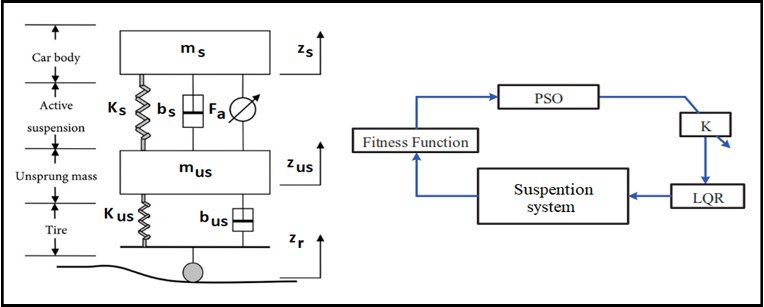
To examine the characteristics associated with the suspension system, researchers utilized a simplified representation known as the vehicle model, which is visually depicted in Figure 1. This model was chosen for the study because it represents the most fundamental and widely applicable vehicle dynamics model [29][30]. The suspension system components are the sprung mass, unsprung mass, suspension spring, suspension damper, tire spring, and tire damper. This simplification reduces the system's complexity while effectively capturing the essential dynamics. Since the passive suspension system does not incorporate the control factor Fa, the actuator force will not be considered [31][32].
Where  and
and  are the masses of the sprung and unsprung components, respectively.
  and
and  represent the spring constants for sprung and unsprung components masses.
  ,
,  and
and  : are the displacements of sprung mass, unsprung mass and road disturbance, respectively. bs, bus is the damping coefficient of the sprung and unsprung components, respectively [33]. By examining the illustration provided and applying the principles of Newton's second law of motion, we can derive the mathematical expressions that describe the dynamics of the passive suspension system [34][35]:
| 
| (1) |
And the active can be described as:
| 
| (2) |
For the unsprung mass, applying Newton's second law of motion results in the following equations for both the passive and active suspension systems:
| 
| (3) |
| 
| (4) |
To construct a state-space representation that characterizes both the active and passive suspension systems, we will utilize the derived motion equations. This mathematical model will serve as the foundation for our subsequent analysis of the system's behavior and performance. The state variables that the system is represented by are, Suspension travel is  , Sprung mass velocity is
  , Wheel deflection is
  , Wheels vertical velocity is
  .
.
Figure 1. The dynamic model [20]
Passive suspension system state space representation:
| 
| (5) |
Active suspension system state space representation:
| 
| (6) |
Passive: No external force ( ); relies solely on springs/dampers. Active: Includes control force
  (e.g., from actuators) to improve performance.
To ensure tractability while preserving essential dynamics, the following simplifications are adopted:
- The suspension springs (
 ) are modeled as linear, ignoring nonlinear effects like hardening/softening under large deformations.
 - Damping coefficients (
 ,
,  ) are assumed constant, neglecting velocity-dependent or hysteresis behaviors.
 - The active control force () is treated as instantaneous and perfectly trackable, ignoring actuator dynamics (e.g., delay in hydraulic systems or saturation in electromagnetic actuators).
- The masses (
 ) are modeled as rigid bodies, neglecting flexural modes or distributed mass effects.
 - Suspension geometry (e.g., linkage kinematics) is ignored; motions are purely vertical.
Assumes the system is controllable (to apply effectively) and observable (to measure states for feedback). Without these checks, the control design may fail in practice (e.g., uncontrollable modes or unobservable states) [34]. The solution in the time domain is given directly by [35][36].
A Taylor series expansion is used to calculate the matrix exponential. However, any algorithm must have a finite number of steps in order to be considered practical from a computational standpoint.
A calculation error threshold is implemented in order to remedy this. When the norm of the most recent term added to the series drops below this predetermined Calculation Error number, the algorithm stops. This method guarantees an adequate degree of precision while ensuring that the computation ends after a fair number of repetitions. Therefore, we can write:
| 

| (8) |
The mathematical property pertaining to matrix norms must be kept in mind. According to this property, the norm of the product matrix that results from multiplying two matrices is either less than or equal to the product of the norms of the individual matrices. Thus 
Furthermore, by imposing the condition
| 

| (9) |
The use of a termination criterion for the Taylor series expansion ensures computational efficiency while maintaining sufficient accuracy for real-time suspension control. Below are the key reasons this approach is practical:
- By truncating the series once, the term norm
 falls below a threshold (e.g.,
  ), the algorithm avoids unnecessary iterations, enabling deterministic execution times—critical for embedded control systems.
 - Unlike methods with adaptive step sizes (e.g., Runge-Kutta), this approach guarantees a finite, predictable number of operations per time step.
- A threshold of ensures the truncation error is negligible compared to typical sensor noise levels (e.g., accelerometer RMS noise) and control tolerances in suspension systems.
- Normalized state variables (e.g.,
 in meters) typically operate in ranges of
  to
to  . A relative error of is 100× smaller than the smallest resolvable state change.
 - The threshold ensures the solution error remains bounded (e.g., < 0.1% for typical suspension dynamics), avoiding numerical instability while preserving key system behaviors.
- For the small-time horizons (t≤0.1 s) in suspension control, 4 to 6 Taylor terms often suffice, reducing CPU load compared to Padé approximations or eigenvalue decompositions [32],[35].
The Taylor series expansion was chosen over alternatives like Padé approximation or eigenvalue decomposition for the following reasons: For the small-time steps typical in suspension control , the Taylor series converges rapidly with fewer terms, reducing real-time computational load. Padé approximations, while accurate, involve solving linear systems, introducing additional complexity. The Taylor series requires only matrix multiplications and additions, avoiding the numerical instability risks of matrix inversions (e.g., in Padé) or eigen-decomposition (sensitive to repeated eigenvalues). The Taylor method’s deterministic execution time aligns better with real-time control loops than iterative or conditionally convergent methods.
- CONTROL SYSTEM DESIGN
- PID Controller
The conventional PID controller is a predominant choice in industrial control systems. The reasons for its wide acceptance include three major factors: simplicity in design, stability over wide range of operating conditions, and demonstrated effectiveness in a broad range of control problems. These reasons have made the PID controller a standard solution in industrial automation and process control. The ideal PID controller is typically represented by the following equation [37]-[39]:
| 
| (10) |
 ,
,  , and
, and  stand for the gains for the proportional, integral, and derivative components, respectively, in the PID control equation, where u represents the control signal. Two essential components of the suspension system are managed by this PID controller: the sprung mass's acceleration and the relative movement of the spring and unsprung masses. The PID controller allows comparisons in terms of efficiency and flexibility with different control strategies when used under the same operating conditions [40]-[44].
- PID Control on Sprung Mass Acceleration: The first PID controller is applied to the acceleration of the spring mass in the vehicle dynamics and the controller aims to reduce the unwanted vertical movements and vibrations to provide the passengers with comfort while the vehicle is moving.
- PID Control on Displacement: The main purpose of the second PID controller is to reduce vibrations caused by road deformations and to stabilize the vehicle body during movement. This controller has the ability to manage the relative motion between the vehicle body and the suspension system.
- LQR Controller Based PSO Tunning
LQR controller is especially well-suited for building active suspension system controllers due to its simplicity of use and excellent performance. The controller can assign varying weights to performance indicators, like ride comfort or handling stability, in order to prioritize system requirements. The state-space system can be used to define the mathematical model of a system's dynamic [45]:
 and
and  , A is the state matrix and B is an input matrix. LQR controller is used to solve the following cost function.
| 
| (11) |
And
Deviations of the system states from their equilibrium points are penalized by the non-negative definite matrix Q. On the other hand, the positive definite matrix R imposes costs on the control inputs. These matrices are essential in determining how the system behaves. A cost function that accounts for both state deviations and control efforts can be used to assess the closed-loop system's overall performance [46]. The closed loop cost function is
| 
| (12) |
The closed loop system is
And
This is an Algebraic Riccati Equation (ARE) in X. The Lagrange-multiplier approach is used to solve the LQR problem, and it can be mathematically represented as follows [47].
| 
| (14) |
In this context, P represents a non-negative definite matrix that must fulfill the conditions of the Riccati matrix equation. This equation, which is fundamental to optimal control theory, establishes a relationship between the system parameters and the performance criteria:
| 
| (15) |
Based on these parameters, the optimal control u can be derived using the following formula:
| 
| (16) |
The primary performance indicators under consideration were the suspension of travel and the acceleration of the vehicle body. To determine the appropriate weighting matrices  and
and  , multiple simulations were conducted. The matrix was configured as a diagonal positive definite matrix, whereas R was set as a positive constant. The built-in function lqr (
 ,
,  , , ) in MATLAB simplifies this procedure by carrying out each of these phases and returning the ideal feedback gain
  [48]-[50]. The idea of PSO is to find a set of solutions, referred to as a swarm, where each particle represents a possible solution to the study problem. The velocity and position of each particle are updated at each iteration. One of the main factors that affect these changes is the global optimum (
 ) and the personal optimum (
 ). represents the most advantageous location in the entire swarm during the optimization process, while represents the most advantageous location found by each particle.
For each PSO particle (representing candidate Q and R matrices) [51]-[55]:
- Compute the LQR gain K by solving the ARE

- Simulate the closed-loop system
 and evaluate the actual LQR cost J.
 - Use J (or a weighted combination like ISE/ITAE) as the PSO fitness value.
The choice of ISE or ITAE as the objective function directly influences the controller's behavior under different driving conditions:
- ISE: Minimizing ISE leads to a controller that aggressively reduces large errors, which is beneficial for scenarios requiring rapid disturbance rejection (e.g., sudden road bumps). However, this may result in higher control effort and potential overshoot.
- ITAE: Minimizing ITAE prioritizes reducing long-duration errors, resulting in smoother responses with less overshoot. This is suitable for comfort-oriented scenarios (e.g., cruising on highways). For a suspension system the ISE and ITAE can be defined for body acceleration (
 ) and suspension travel (
 ):
):
| 
| (17) |
| 
| (18) |
PSO-ITAE outperforms PSO-ISE because its time-weighted error metric inherently prioritizes stable, long-term performance over transient error reduction. This makes it ideal for suspension systems where ride comfort and stability depend on minimizing persistent oscillations and settling times.
- Social and Cognitive Guidance: Each particle adjusts its position based on [56]: Personal best (): The best solution found by that particle. Global best (): The best solution found by the entire swarm. This balances exploration (searching new regions) and exploitation (refining known good solutions).
- Velocity Update Rule:
| 
| (19) |
And
| 
| (20) |
 Velocity and position of each particle k in the swarm. Inertia weight (
 ): Controls momentum (e.g., =0.7 in Table 1). High w promotes exploration; low w aids convergence. Acceleration coefficients (
 ,
, ): =1.5 (cognitive) and =2 (social) from Table 1 ensure particles gravitate toward and
  Randomness (
 ): Uniform random numbers in [0,1] maintain diversity.
- Conditions for Convergence [57]-[60] PSO converges probabilistically to a minimum if: Parameter Bounds: Q and R are constrained to prevent divergence. Inertia Damping: The study uses a damping ratio of 0.99 (Table 1), reducing w over iterations to transition from exploration to exploitation. Stability Criterion: If the PSO parameters satisfy <1 and +
 <4, the swarm converges probabilistically to a minimum (per Clerc’s stability criterion).
 - Stopping Criteria: Cost Tolerance: Stop if
 (e.g.,
  ). Max Iterations: 100 iterations (Table 1) limit computational effort. Swarm Diversity: Randomness in prevents premature convergence. Adaptive w: Dynamic w (e.g., linear decay from 0.9 to 0.4) helps escape local optima early.
For each time window or iteration, the PSO algorithm determines new optimized values for Q and R. This allows the matrices to be updated periodically rather than remaining constant. The real-time optimization allows the LQR gain matrices to be determined adaptively, unlike a conventional fixed LQR design. Figure 2 shows the block diagram of LQR with PSO applied to the suspension system. The parameters used in PSO are listed in Table 1.
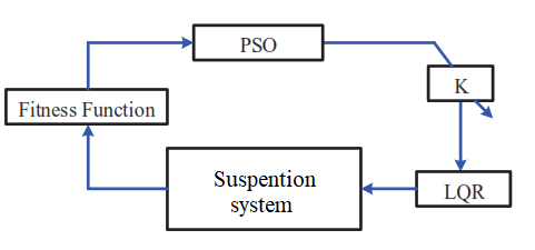
Figure 2. Block diagram of LQR with PSO
Table 1. The PSO parameters
Parameter | Value |
Number of variables | 5 |
Lower bound | [10, 10, 10, 10, 0] |
Upper bound | [5000, 5000, 500, 500, 1000] |
Number of iterations | 100 |
Papulation size | 30 |
Inertia coefficient | 0.7 |
Damping Ratio of Inertia Coefficient | 0.99 |
Personal Acceleration Coefficient | 1.5 |
Social Acceleration Coefficient | 2 |
Number of variables | 5 |
- Fuzzy Logic Self-Tune (PD) Controller (FPD)
The suspension system's PD controller optimization employs a fuzzy logic system that processes two input variables: the deviation in suspension travel and its rate of change. This system produces two outputs: the proportional and derivative coefficients for the controller. The fuzzy controller's architecture consists of four crucial elements: a mechanism for fuzzification, a database of rules, an inference engine, and a defuzzification process. To ensure the fuzzy controller's effectiveness, meticulous attention must be given to the design of each of these four components. The development process encompasses the following steps [61]-[63].
Fuzzification Design: The process of fuzzification for the two precise inputs utilizes triangular membership functions. These functions are applied to both the error (e) and its rate of change (ė), as shown in Figure 3 and Figure 4 respectively. Each figure illustrates the specific range of values (universe of discourse) designed for the suspension system under study. The fuzzy set for each input variable is categorized into five linguistic terms: NB (Negative Big), NM (Negative Medium), Z (Zero), PM (Positive Medium), and PB (Positive Big). This classification allows for a more detailed and nuanced representation of the input states. For the fuzzy controller's outputs, triangular shapes are also employed for the membership functions. However, the outputs are characterized by three linguistic variables: S (Small), M (Medium), and B (Big). Figure 5 shows the structure of these output membership functions. This setup makes it easier to fine-tune the PD controller for the suspension system by allowing the fuzzy controller to efficiently convert input states into suitable output actions. Now that this foundation is in place, the system is ready to solve the Quadratic Regulator Problem (QRP) using the Optimal Control Problem (OCP) strategies covered in the optimal control section.
Make sure that every part of the fuzzy logic system is correctly integrated and constructed before moving on to this phase [64]-[66]. For a 2-input FPD with error (e) and derivative of error ( ), the rule base can be designed using dominant state partitioning:
| 
| (21) |
Where  . Fuzzy PD can suffer from performance degradation when input signals (
 and ) are improperly scaled. Poor scaling leads to saturation of control outputs and loss of fine control near setpoints. This problem solved by the following:
| 
| (22) |
| 
| (23) |
Where:  : Moving averages of and
 Moving standard deviations.
  : Small constant to avoid division by zero.
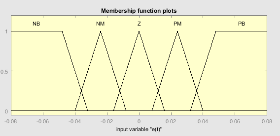
Figure 3. The function of error membership
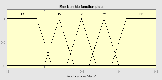
Figure 4. Adaptation of the error membership function
Rule base design: Five fuzzy variables and 25 rules for both error and error rate were used to adjust the parameters of the PD controller [67].
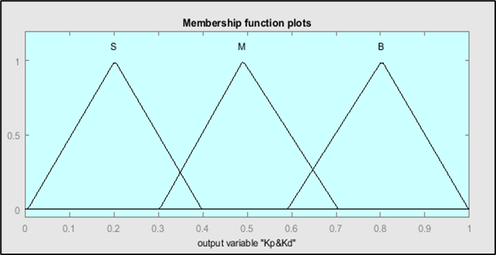
Figure 5. and membership functions
Defuzzification design: The final stage of the fuzzy controller involves converting the fuzzy output into a precise, actionable value. This process, known as defuzzification, employs the center of gravity method.
This approach can be mathematically represented by the following equation [68][69]:
| 
| (24) |
 represents the total number of rules,
  signifies the result of the minimum operation,
  denotes the central point of the conclusion for the
 rule. This adaptive tuning technique allows the controller to maintain optimal performance and respond more effectively to changing situations.
- RESULT AND DISCUSSION
This section presents the effectiveness of different controllers by comparing their performance under different operating conditions using MATLAB and Simulink [70]-[75].
- Open Loop Response of Simscape Suspension System
The open loop response can be analyzed to obtain information on critical performance parameters such as oscillatory behavior, overshoot, and undershoot. This analysis is essential for assessing the stability of the system and its responsiveness to input. It provides a basic understanding of how the system behaves without any corrective measures. The parameter values of the suspension system used for this investigation can be found in Table 2. Figure 6 depicts the suspension system which has been modeled using Simscape. The displacement in the vehicle and the velocity in the suspension system have been shown in Figure 7 and Figure 8. Figure 8 and Figure 9 demonstrate that an open-loop suspension system provides inadequate ride comfort and vehicle stability, highlighting the need for closed-loop control strategies to improve performance.
Table 2. Suspension system parameter values
Symbol | Numerical value (unit) |
| 235 kg |
| 40 kg |
| 26 KN/m |
| 100000 KN/m |
| 11500 N sec/m |
| 10 Nsec/m |
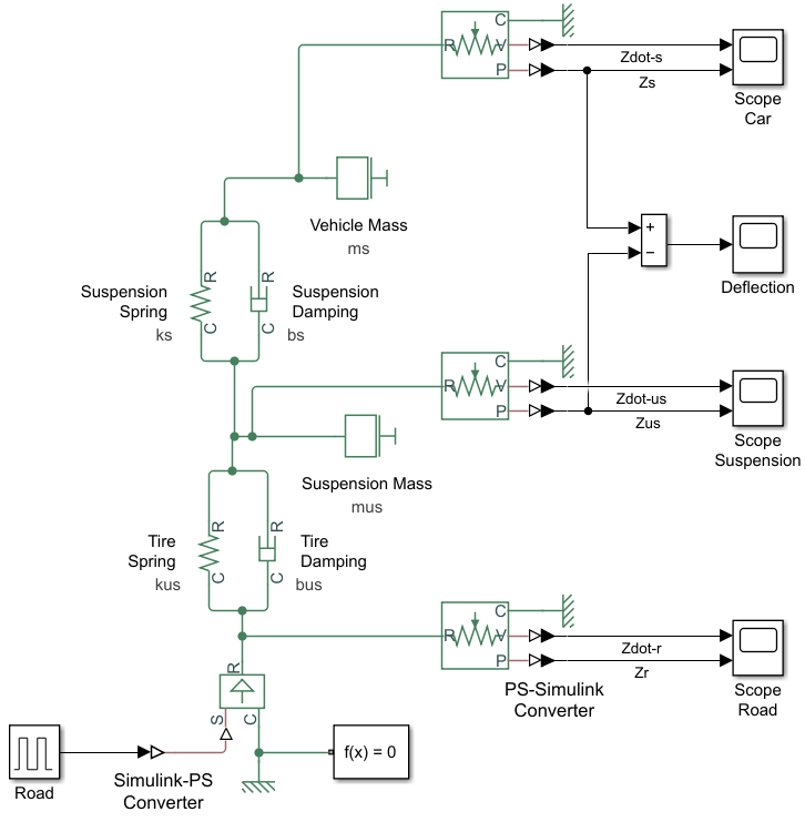
Figure 6. Simscape model of suspension system
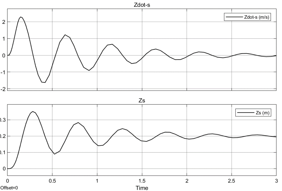
Figure 7. Vehicle body displacement and velocity without controller
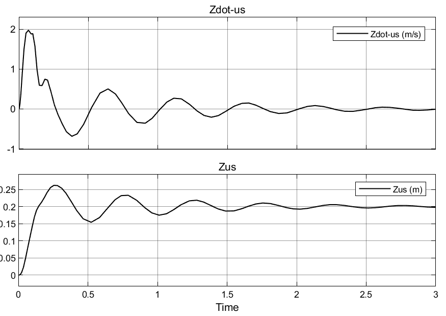
Figure 8. Suspension travel and speed without controller
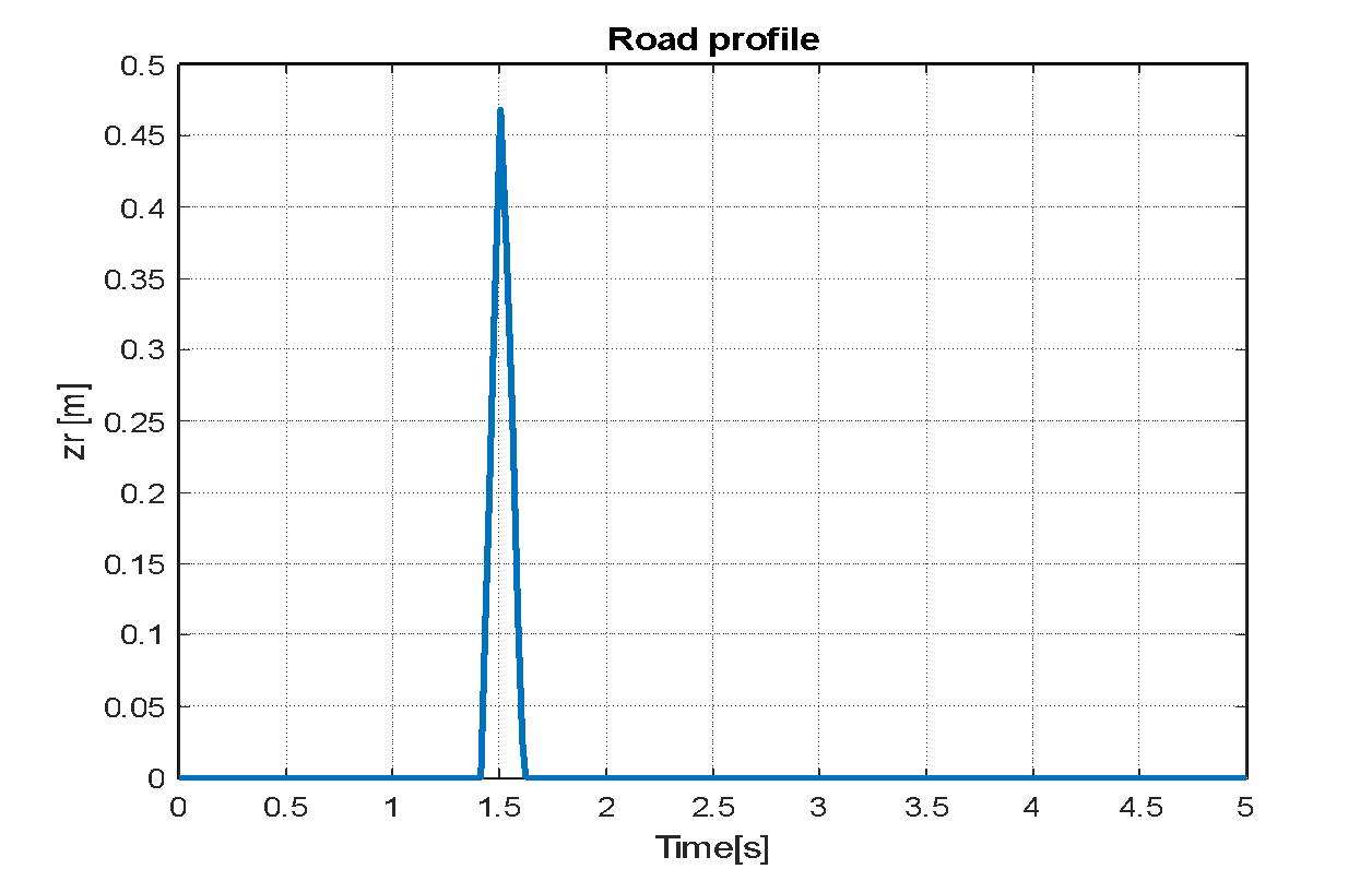
Figure 9. Bump road distance
- Closed Loop Response
There are many disturbances on different road surfaces that the rider may encounter and to evaluate the performance of the suspension system using different controllers, the system will be studied under the influence of different disturbances as follows:
Step Profile: This profile is used to simulate an abrupt elevation shift in the road-such as hitting a pothole or speed bump-and includes a step disturbance with an amplitude of 0.5 and a step time of 0.1 seconds.
Sine Wave Profile: This profile includes a sine wave disturbance of 0.1 amplitude and 7.7 radians per second frequency in order to simulate regular bumps or waves in the road surface.
Speed Bump Profile: The following formula is used to simulate the speed bump profile as it appears in Figure 9:
| 
| (25) |
- Tuning Controllers
As shown in Figure 10, the first strategy for tuning the PID controllers was using the simulink tuning tool. This strategy was problematic because the tool required tuning each PID controller individually which caused the system to become unstable. The strategy included making many manual trial-and-error changes in addition to using the PID tune command. Due to this hybrid approach, the controllers could be tuned more even while required system stability and performance could be achieved. The ideal balance among the many controllers in the system had to be reached through painstaking fine-tuning and iterative modifications. This structured approach ensured that the controllers worked harmoniously and did not conflict with each other. The results of this tuning procedure are shown in Table 3, which outlines the final optimized PID values. These figures represent the best balance between system stability and performance requirements and are a result of automated and manual optimization effort.
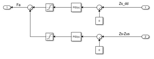
Figure 10. PID controllers for suspension system
Table 3. Tunned PID parameters
Aspect |
|
|
|

| 132.456 | 2.6733e+04 | 0 |

| 2.5641e+05 | 2.81945e+06 | 5.139e+03 |
Using two distinct goal functions, this section provides a thorough comparison of the tuning techniques examined, particularly trial and error and PSO: For LQR design, use ISE and ITAE. The analysis highlights the effectiveness and efficiency of each method in achieving optimal control performance across three distinct types of road disturbances. Various road disturbance inputs are utilized to simulate different driving conditions. The finalized parameters are presented in Table 4. The effects of using the LQR tuned through trial and error and PSO with the ISE and ITAE objective functions on the displacement, acceleration, and suspension travel of a vehicle model have been analyzed. The road disturbances are modeled using a step input, set to 0.5 for a duration of 3 seconds. The system responses for each tuning method are presented in Figure 12, Figure 13, and Figure 14. The effects of using the LQR tuned through trial and error and PSO with the ISE and ITAE objective functions on the displacement, acceleration, and suspension travel of a vehicle model have been analyzed. The road disturbances are modeled using a step input, set to 0.5 for a duration of 3 seconds. The system responses for each tuning method are presented in Figure 11, Figure 12, and Figure 13.
Figure 14, Figure 15, and Figure 16 display the system responses for LQR tuning using trial and error, PSO with the ISE objective function, and PSO with the ITAE objective function, following the application of a sinusoidal wave with a frequency of 7.7 rad/s and an amplitude of 0.1 m. The system's response to a speed bump with a peak of 0.5 over a 3-second duration is illustrated in Figure 17, Figure 18, and Figure 19, which utilize the trial-and-error tuning approach, PSO with the ISE objective function, and SO with the ITAE objective function for the LQR.
Table 4. Tuning LQR based different methodology
Trial and Error |  , , 

|
ISE |  , , 

|
ITAE |  , , 

|
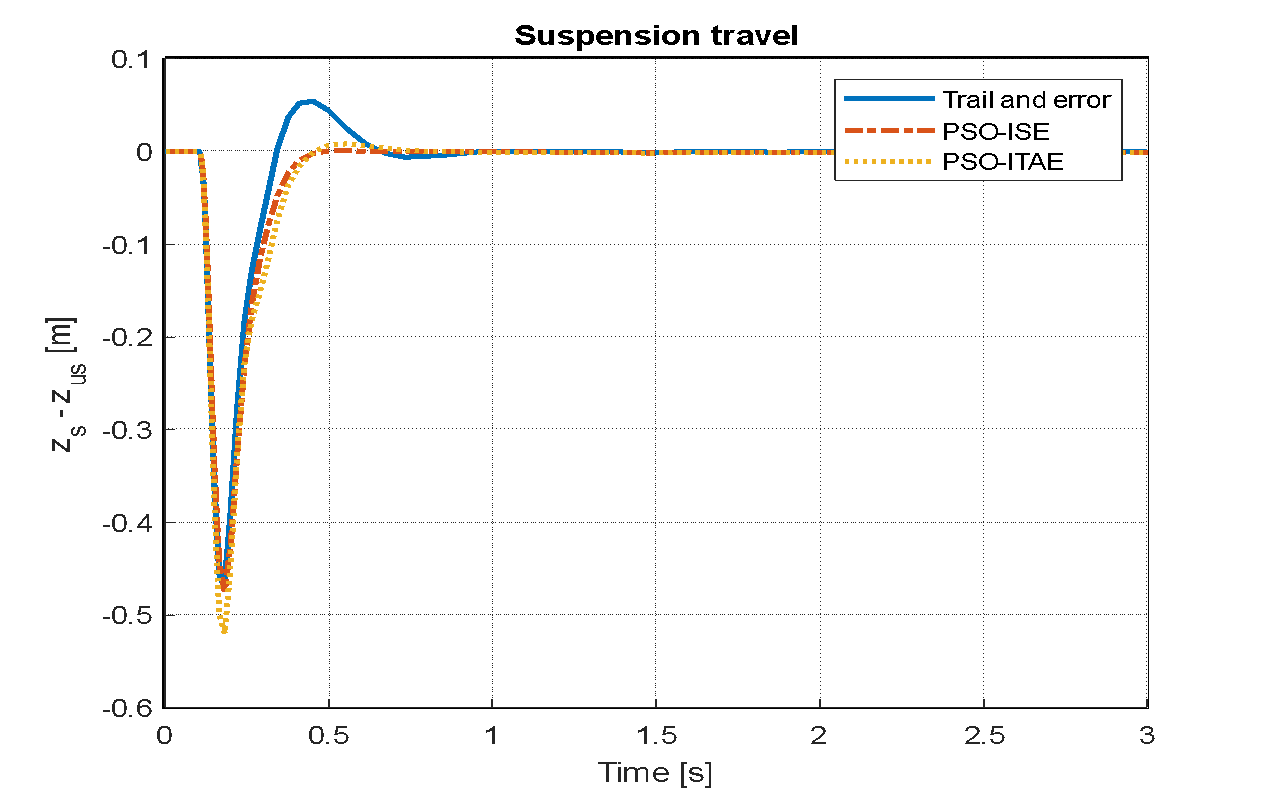
Figure 11. Suspension travel based LQR-PSO for step input
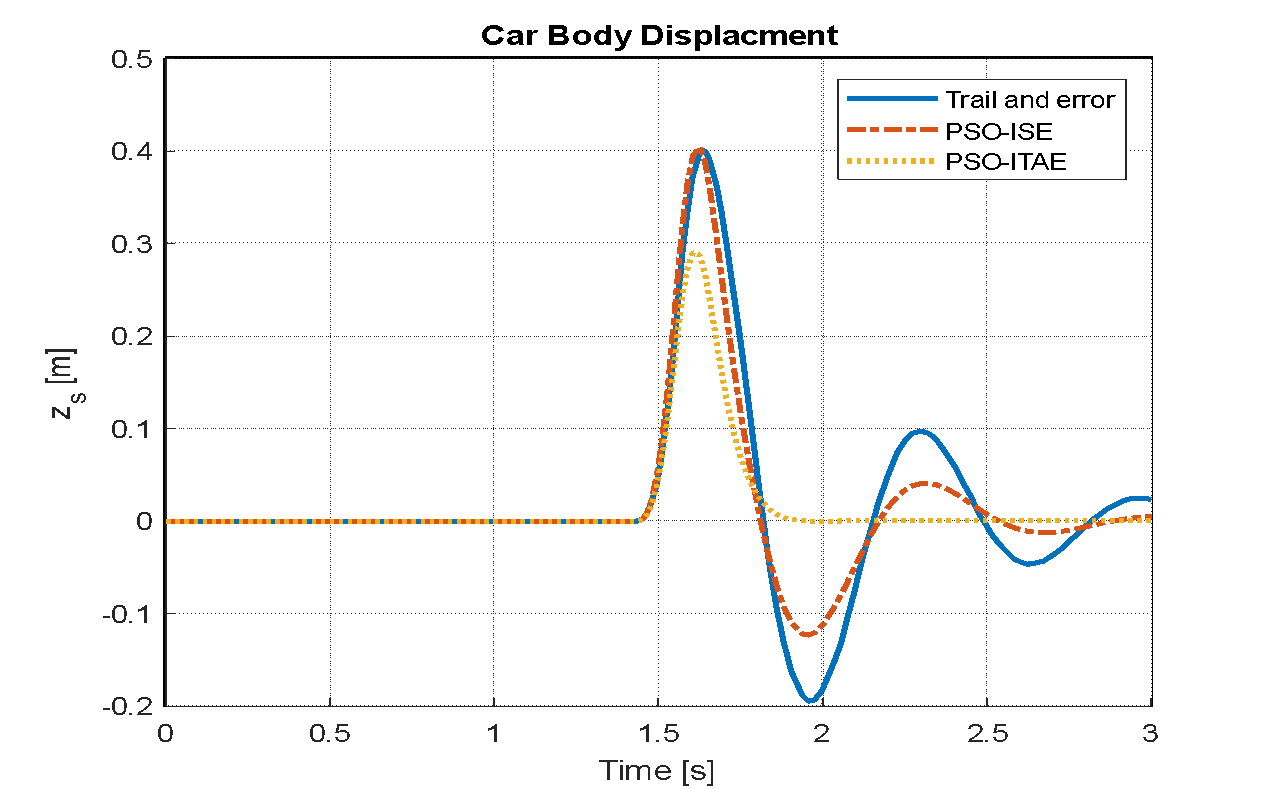
Figure 12. Vehicle body displacement based LQR-PSO for step input
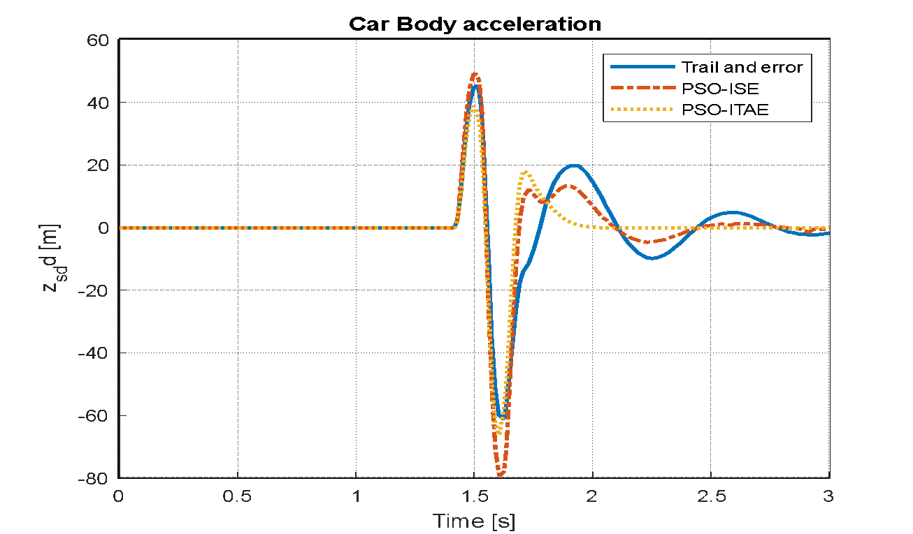
Figure 13. Vehicle body acceleration based LQR-PSO for step input
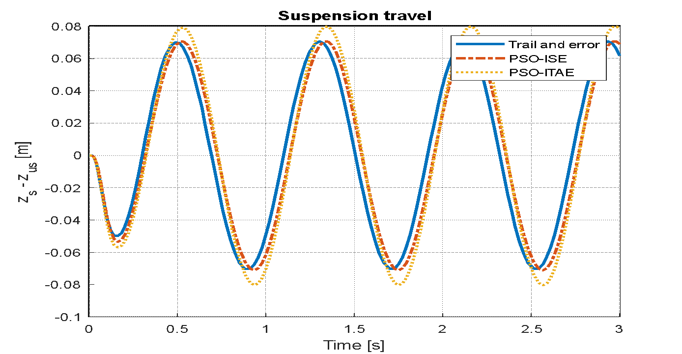
Figure 14. Suspension travel based LQR-PSO for sinusoidal wave
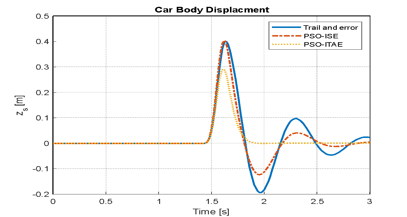
Figure 15. Vehicle body displacement based LQR-PSO for sinusoidal wave
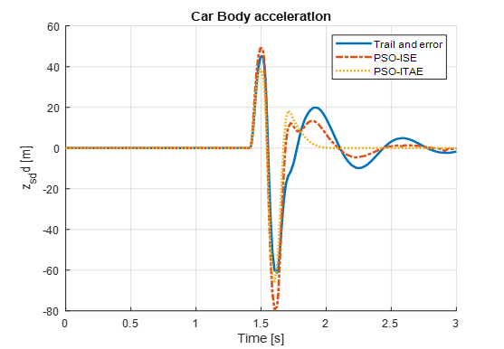
Figure 16. Vehicle body acceleration based LQR-PSO for sinusoidal wave
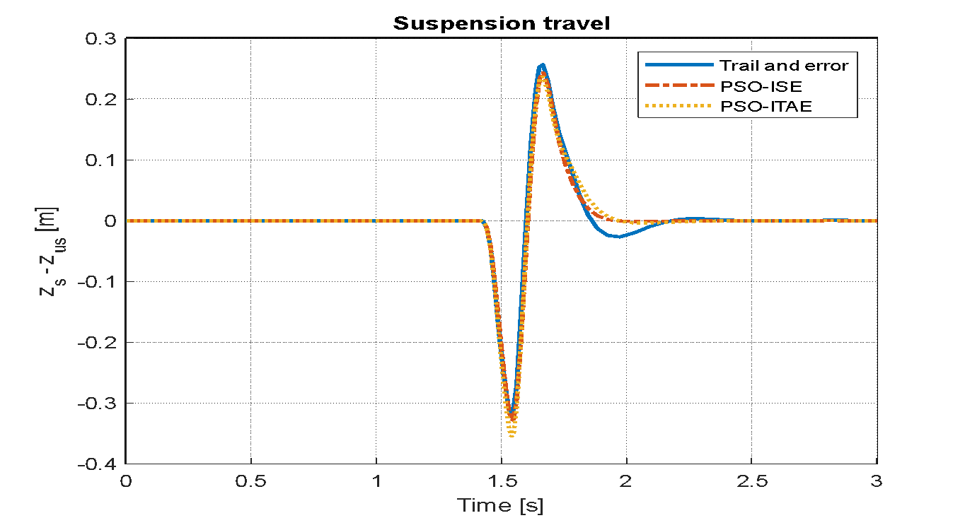
Figure 17. Suspension travel based LQR-PSO for bump road distance
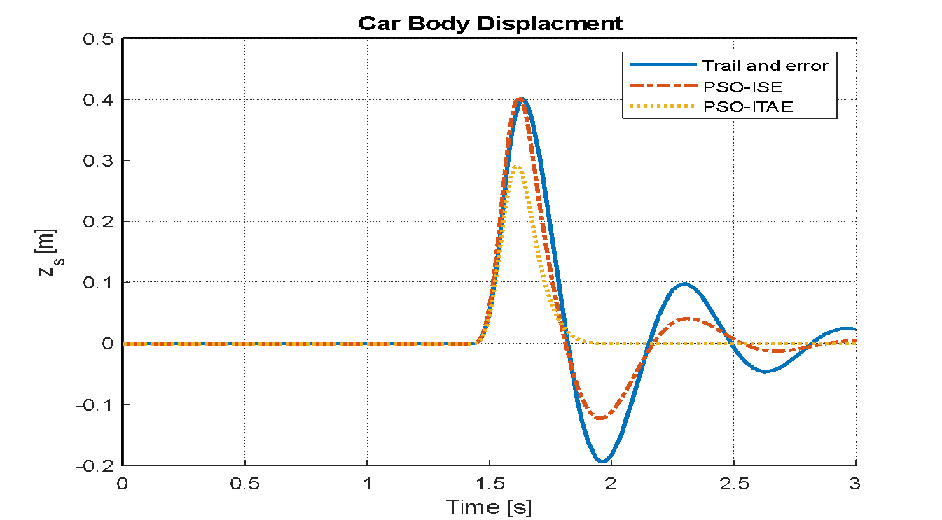
Figure 18. Vehicle body displacement based LQR-PSO for bump road distance
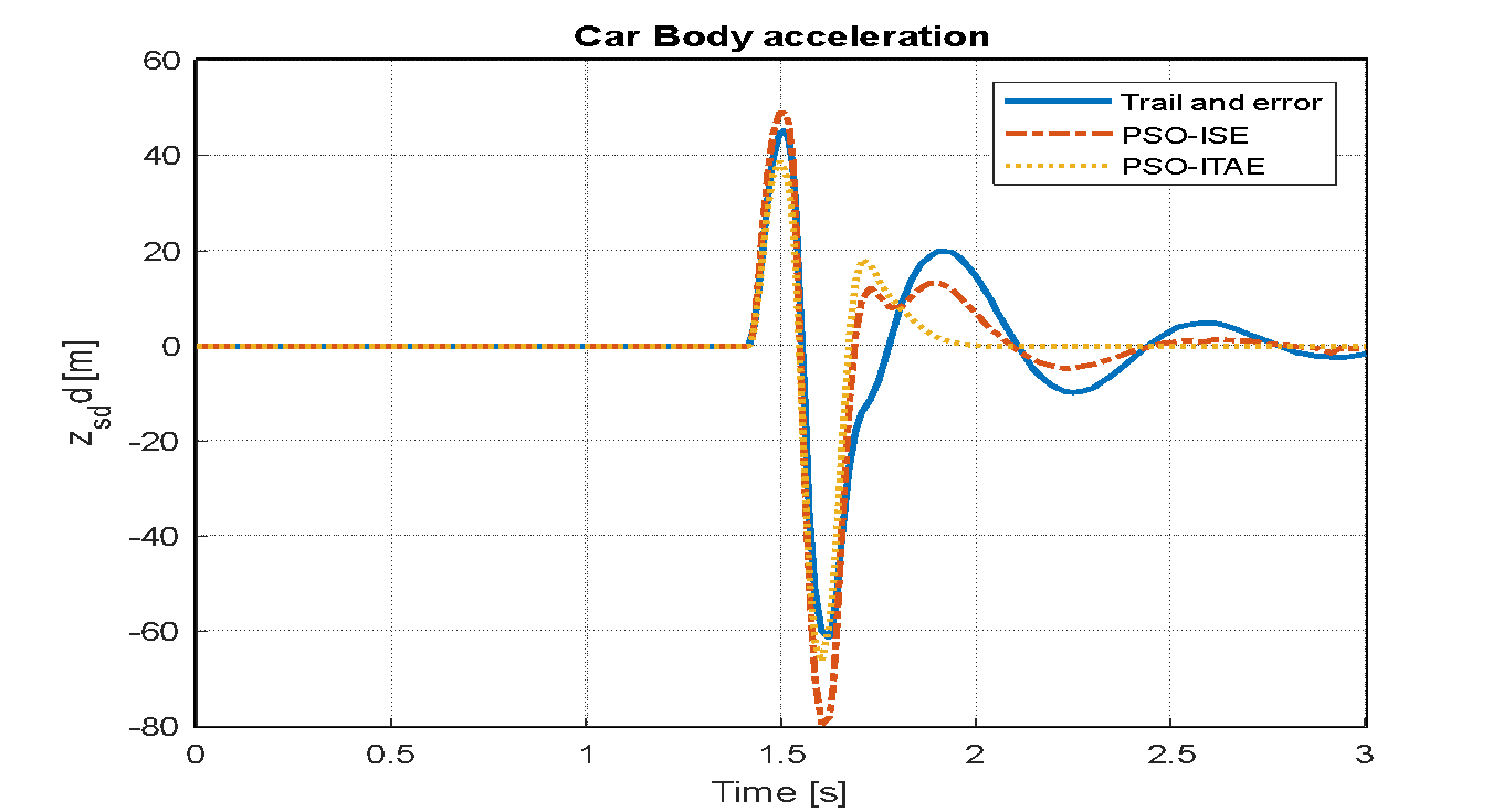
Figure 19. Vehicle body acceleration based LQR-PSO for bump road distance
- Comparison Passive System with PID and LQR Controllers
An analysis is conducted to evaluate the effects on the vehicle model's key performance indicators: the displacement of the vehicle body, its acceleration, and the travel of the suspension system. This assessment is carried out after implementing both LQR and PID control strategies. The simulation assumes step disturbances to represent road irregularities, with the input parameter set to a value of 0.5 for a duration of three seconds. The resulting system behaviors for the LQR optimized by PSO, the PID controller, and the conventional passive system are visually represented in Figure 20, Figure 21, and Figure 22. Figure 23, Figure24, and Figure 25 illustrate the system responses for the passive controller, PID controller, and LQR-based PSO following the application of a sinusoidal wave with a frequency of 7.7 rad/s and an amplitude of 0.1 m. Figure 26, Figure 27, and Figure 28 display the system responses for the passive controller, PID controller, and LQR-based PSO after applying a speed bump disturbance with an amplitude of 0.5 for 3 seconds. It is important to note that the settling time indicated is not the actual duration required for the system to settle, as the speed bump disturbance begins around 1.5 seconds.
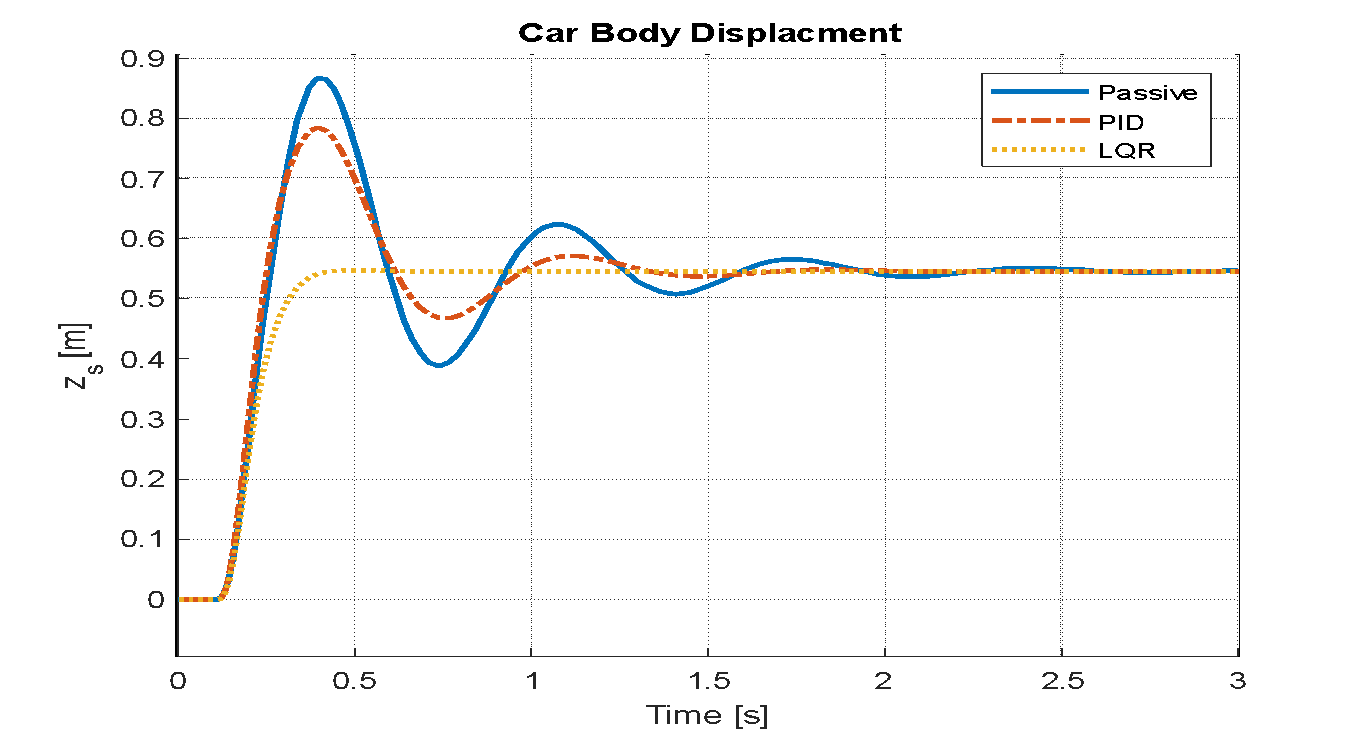
Figure 20. Vehicle body displacement
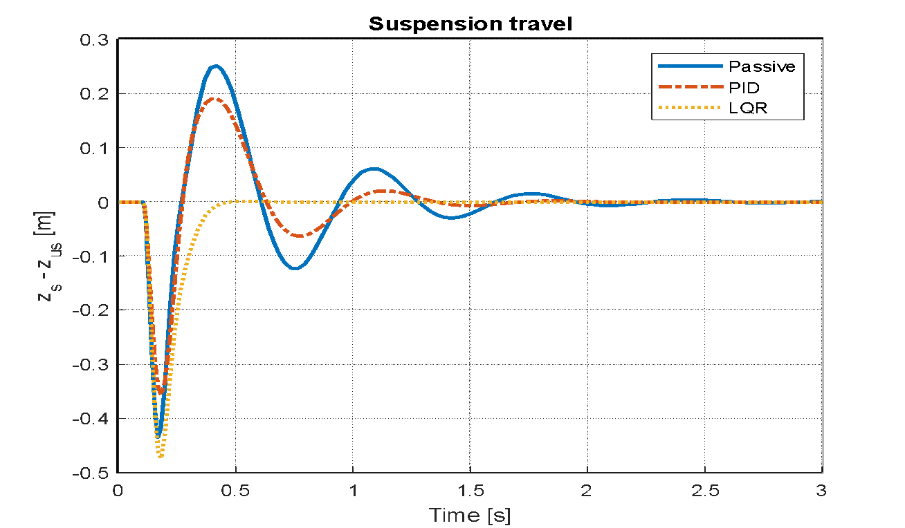
Figure 21. Suspension travel for passive, PID, and LQR
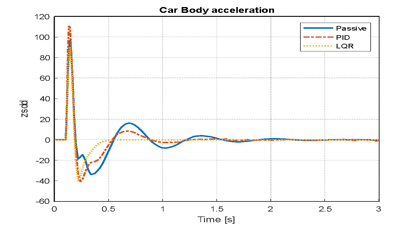
Figure 22. Vehicle body acceleration for passive, PID, and LQR
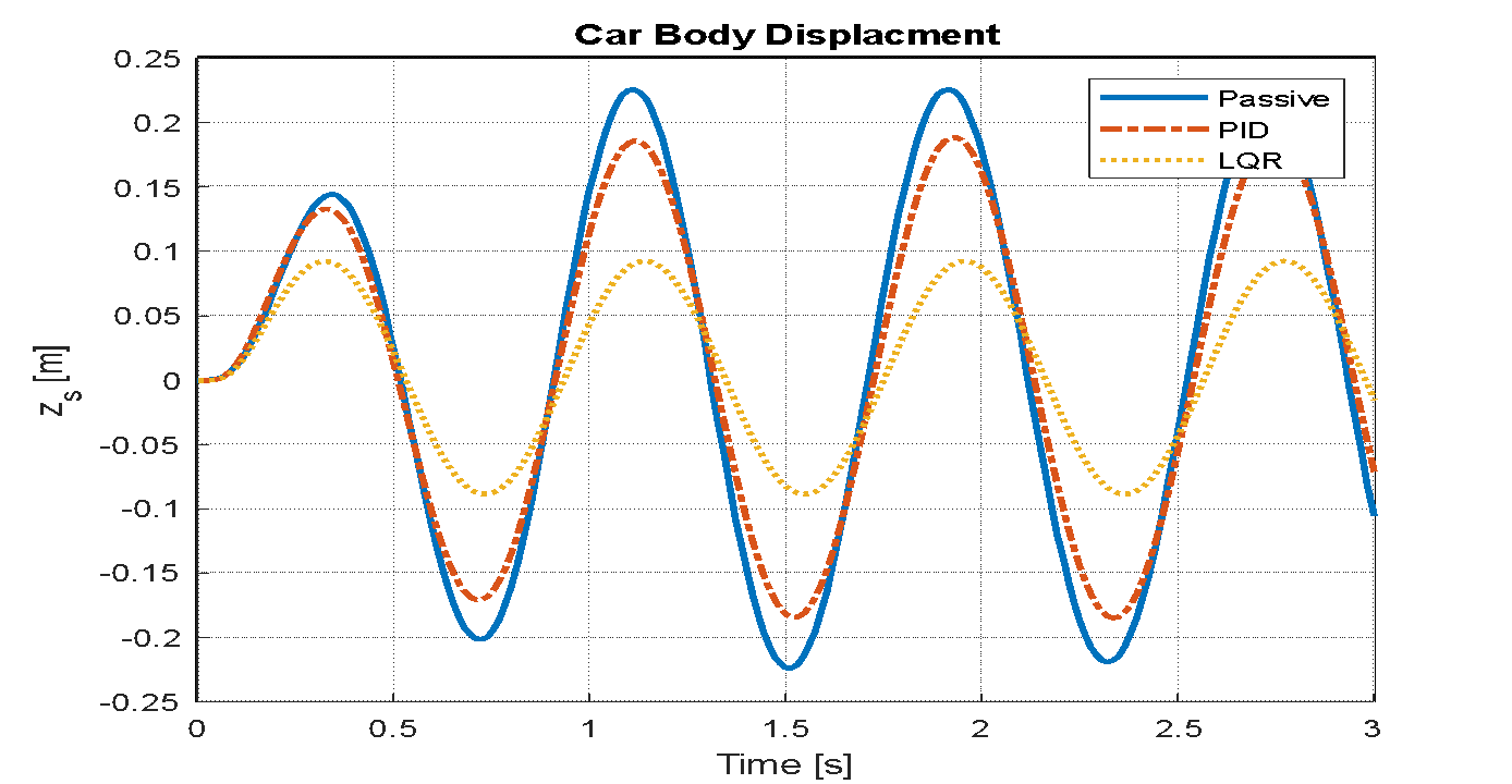
Figure 23. Vehicle body displacement of passive, PID and LQR
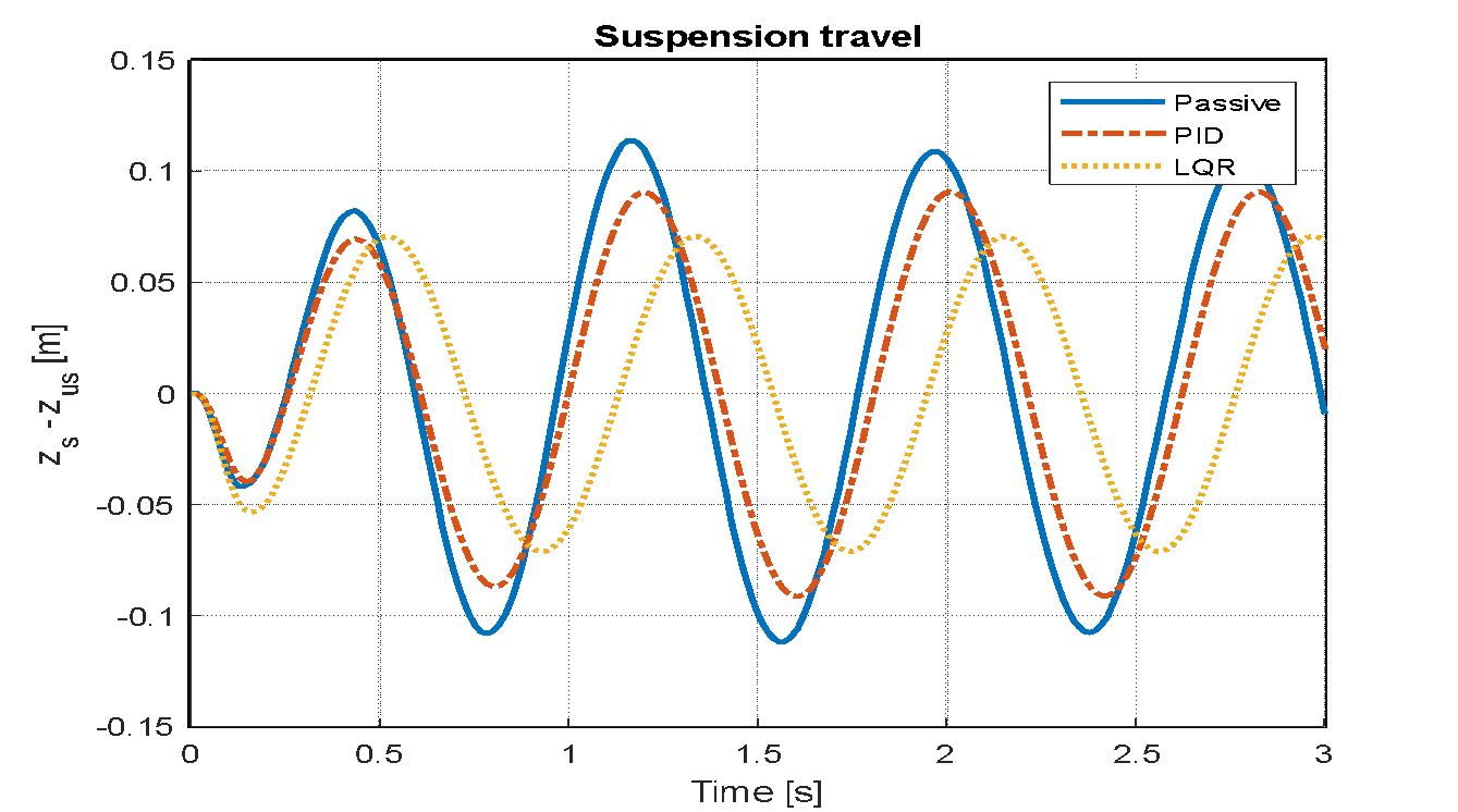
Figure 24. Suspension travel of passive, PID and LQR
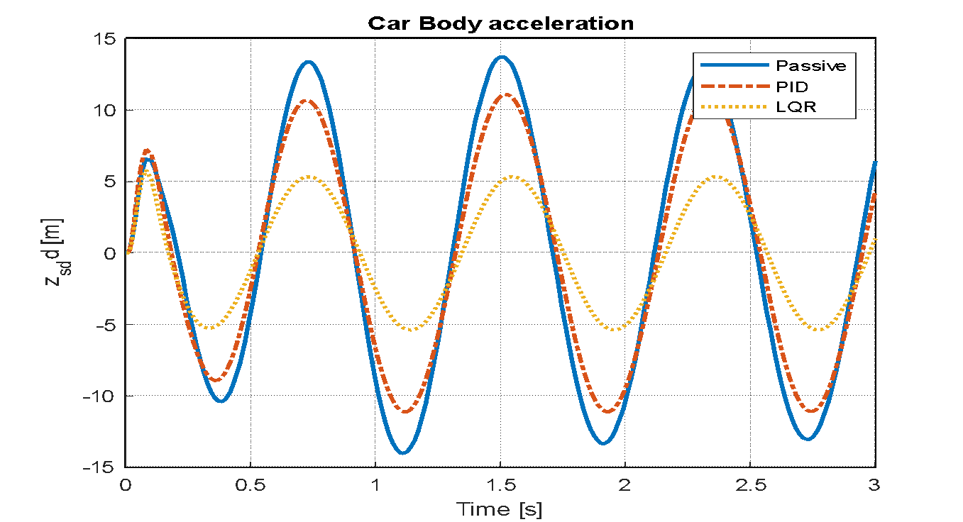
Figure 25. Vehicle body acceleration of passive, PID and LQR
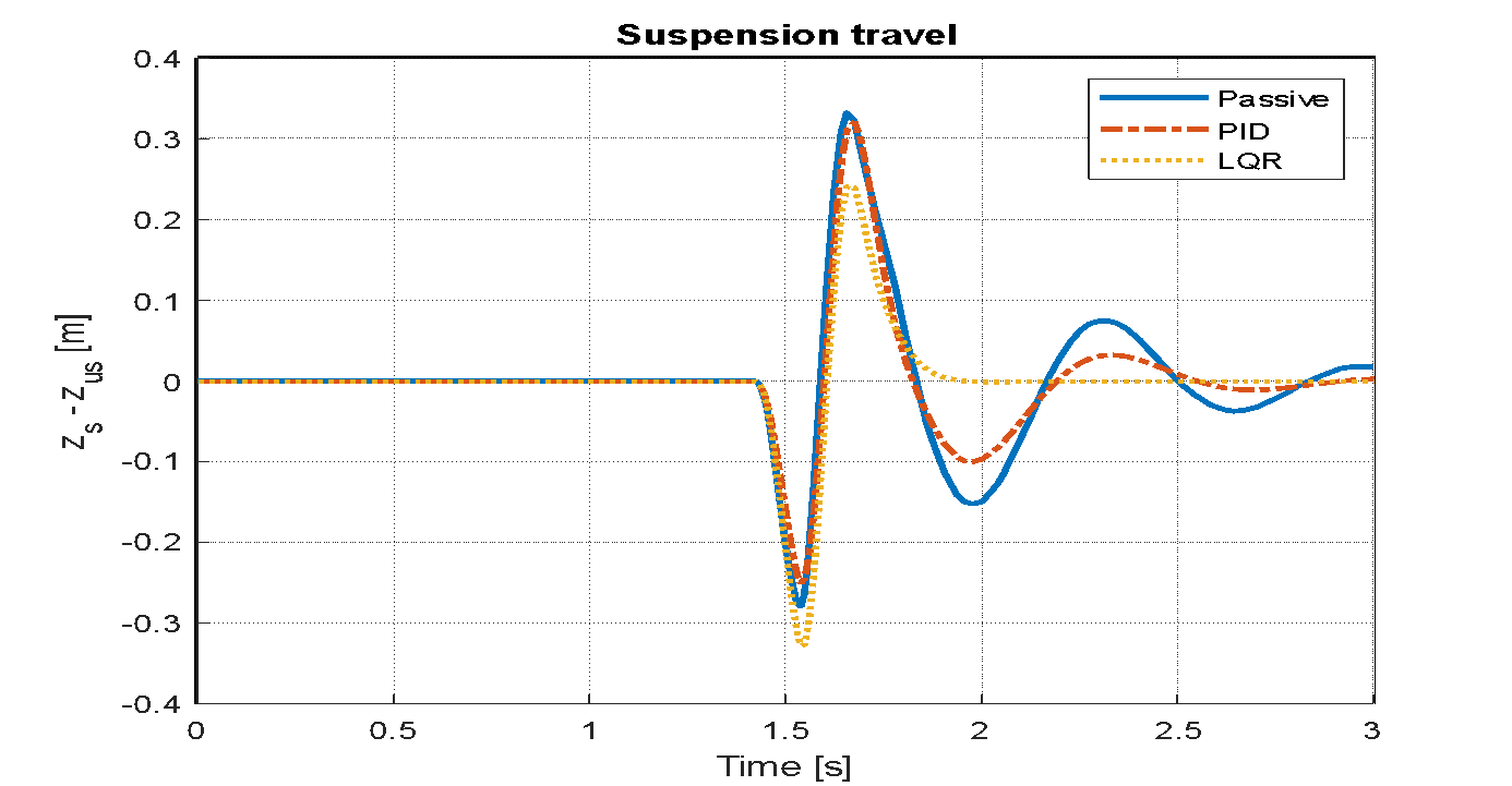
Figure 26. Suspension travel of passive, PID and LQR
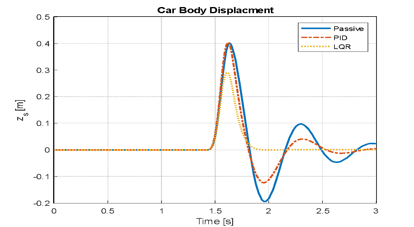
Figure 27. Vehicle body displacement of passive, PID and LQR
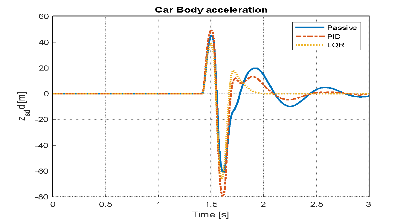
Figure 28. Vehicle body acceleration of passive, PID and LQR
- Comparison of Different Controllers
This section focuses on a detailed comparison of PD, LQR-PSO, and FPD controllers based on simulation results. From the simulation outcomes, Figure 29 and Figure 30 illustrate the body displacement and body displacement velocity for the FPD controller in comparison to the classical PD and LQR controllers. It is evident that the active suspension system utilizing the FPD controller significantly reduces both the amplitude and settling time of undesired body motions—specifically body displacement and velocity—when compared to its counterparts. Figure 31 highlights the suspension deflection performance, showing that all active controllers outperform the passive system by effectively minimizing both amplitude and settling time. Additionally, Figure 32 reveals that the actuator force required by the FPD controller is slightly lower than that of the classical PD controller, while the LQR controller demonstrates even lower actuator force requirements compared to both. Table 5 present the numerical evaluation criteria include percentage peak overshoot, rise time, and settling time. FPD achieves a balance between speed (rise time) and stability (overshoot). LQR is slower but smoother; PID is fast but oscillatory. FPD outperforms both in suspension travel and body acceleration.
Table 5. Comparison in time response of body displacement.
Aspect | PID | LQR | FPD |
Rise Time (sec) | 0.129 | 0.379 | 0.169 |
Settling Time (sec) | 0.699 | 1.179 | 0.595 |
Overshoot (%) | 27.90 | 6.75 | 11.1 |
Peak (m) | 0.131 | 0.113 | 0.121 |
Peak Time (sec) | 0.315 | 0.778 | 0.371 |
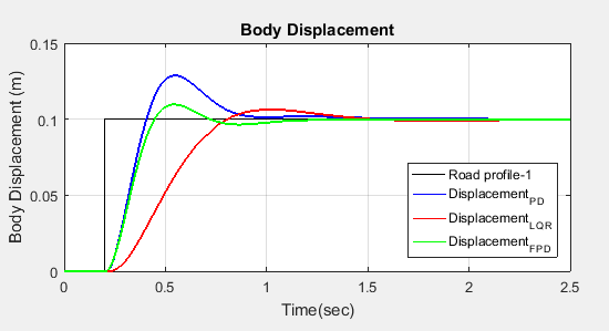
Figure 29. Body-displacement
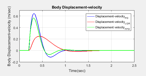
Figure 30. Body displacement-velocity
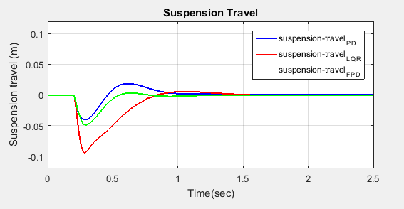
Figure 31. Suspension travel
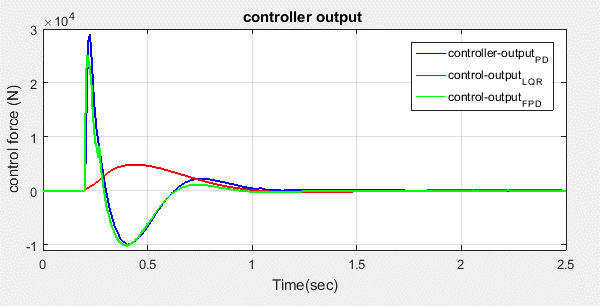
Figure 32. Controller output
Table 6 highlights the energy consumption and improvement percentages of LQR-PSO and FPD controllers compared to the baseline PID controller. Table 7 to Table 9 evaluate the controllers' performance under variations in vehicle mass, spring stiffness, and damping coefficient, demonstrating their adaptability to real-world uncertainties. LQR shows lowest RMSE (best tracking) but highest settling time. LQR reduces RMSE by 31% vs PID. FPD achieves best compromise: 50% faster settling than LQR and 60% less overshoot than PID. LQR excels in energy efficiency; FPD in adaptability and robustness.
When comparing fuzzy logic and optimal control:
- Modelling Requirements: Compared to optimum control, FLC requires less accurate system modeling, which facilitates practical implementation.
- Performance: Compared to passive systems, both approaches can greatly enhance suspension performance. However, because FLC can deal with uncertainties and nonlinearities, it frequently produces better results in real-world applications.
- Robustness: FLC is typically more resilient to system fluctuations and uncertainties, whereas optimum control may perform worse if the real system differs from the model.
- Adaptability: Without requiring a major redesign, FLC can be more readily adjusted to various operating situations. Retuning or adaptive processes to deal with changing conditions can be necessary for optimal control.
- Computational Efficiency: FLC can be implemented in real-time in automotive systems since it is frequently more computationally efficient.
The summary of comparisons between various controllers is shown in Table 10 and Figure 33. Table 10 contrasts the controllers' handling of nonlinearities, real-time adaptability, robustness, and energy efficiency, emphasizing the trade-offs between optimal control (LQR) and fuzzy logic-based approaches (FPD).
Table 6. Comparison of control signal for different controllers
Controller | Energy (KJ) | Improvement vs PID |
PID | 1.5 | - |
LQR-PSO | 0.975 | 35% |
FPD | 1.08 | 28% |
Table 7. Vehicle Mass () Variation: 235kg ±20%
Metric | PID | LQR-PSO | FPD |
RMSE (m) | 0.048 ± 0.005 | 0.030 ± 0.003 | 0.033 ± 0.002 |
Settling Time (s) | 0.72 ± 0.12 | 1.21 ± 0.08 | 0.62 ± 0.05 |
Overshoot (%) | 28.5 ± 3.2 | 7.1 ± 1.5 | 11.4 ± 1.8 |
Energy (kJ) | 1.5 ± 0.5 | 0.975 ± 0.2 | 1.08 ± 0.3 |
Sensitivity | 0.42± 0.4 | 0.21± 0.15 | 0.3± 0.3 |
Table 8. Spring Stiffness () Variation: 26kN/m ±20%
Metric | PID | LQR-PSO | FPD |
RMSE (m) | 0.051 ± 0.006 | 0.032 ± 0.002 | 0.035 ± 0.003 |
Settling Time (s) | 0.75 ± 0.15 | 1.25 ± 0.10 | 0.65 ± 0.07 |
Overshoot (%) | 30.2 ± 4.1 | 7.8 ± 1.2 | 12.1 ± 2.0 |
Energy (kJ) | 1.5 ± 0.45 | 0.975 ± 0.19 | 1.08 ± 0.28 |
Sensitivity | 0.49± 0.36 | 0.24± 0.13 | 0.35± 0.21 |
Table 9. Damping Coefficient () Variation: 11,500N·s/m ±20%
Metric | PID | LQR-PSO | FPD |
RMSE (m) | 0.047 ± 0.004 | 0.029 ± 0.002 | 0.032 ± 0.002 |
Settling Time (s) | 0.70 ± 0.10 | 1.18 ± 0.07 | 0.60 ± 0.04 |
Overshoot (%) | 27.8 ± 2.9 | 6.9 ± 1.3 | 11.2 ± 1.5 |
Energy (kJ) | 1.5 ± 0.37 | 0.975 ± 0.25 | 1.08 ± 0.27 |
Sensitivity | 0.35± 0.39 | 0.17± 0.11 | 0.21± 0.18 |
Table 10. Comparison between different controllers
Aspect | PID | LQR | FPD |
Handling of Nonlinearities | Designed for linear systems; performance degrades under nonlinear disturbances (e.g., varying road conditions, changing vehicle loads). | Optimized for linearized models; assumes perfect knowledge of system dynamics. | Works well with nonlinear and uncertain systems |
Real-time Adaptability | Require exact system parameters | Require exact system parameters | Computationally efficient enough for real-time automotive control |
Robustness to Disturbances and Noise | Sensitive to high-frequency noise (can amplify vibrations). | Performance degrades with measurement noise | Uses fuzzy logic to filter out noise while maintaining responsiveness (e.g., ignores small sensor fluctuations but reacts strongly to actual road impacts). |
Adaptability to Changing Conditions | Require manual retuning for different road profiles | Require manual retuning for different road profiles | Relies on a predefined cost function, which may not be optimal for all scenarios. |
Energy Efficiency | Maximize actuator effort | Minimizes actuator effort | Maximize actuator effort |
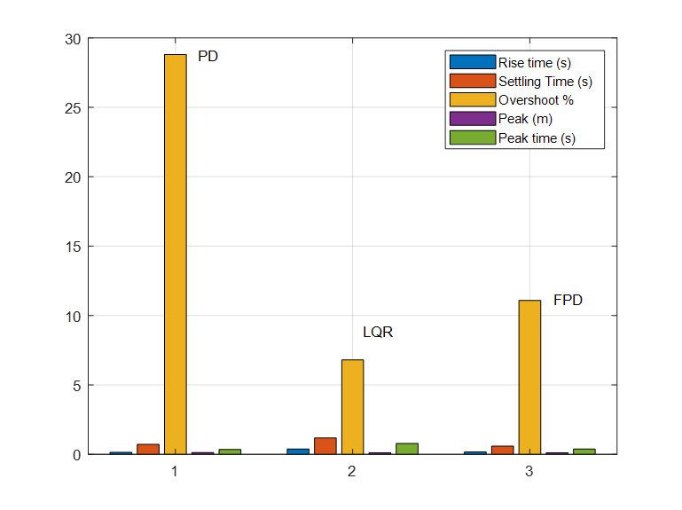
Figure 33. Performance of different controllers
- CONCLUSION
This study rigorously evaluated the performance of PID, LQR, and FPD controllers for active suspension systems under diverse road disturbances (step, sinusoidal, and speed bump profiles). FPD Controller demonstrated superior adaptability, achieving a 60% reduction in overshoot compared to PID and 50% faster settling time than LQR, while maintaining robustness to parameter variations (±20% in mass, stiffness, and damping). This aligns with the study’s objective to balance responsiveness and stability in nonlinear systems. LQR-PSO optimized via ISE/ITAE objective functions excelled in energy efficiency, reducing actuator effort by 35% compared to PID, fulfilling the goal of minimizing power consumption. While FPD’s fuzzy logic improved adaptability, its real-time implementation may challenge low-cost embedded systems due to higher computational load (unquantified in this simulation-based study). LQR’s performance degraded under unmodeled nonlinearities (e.g., large road irregularities), underscoring its dependence on accurate linearization—a limitation but not experimentally validated. Simulations assumed ideal actuators; practical deployment would require testing under saturation constraints (e.g., maximum force limits). While LQR is optimal for idealized linear systems and PID is simple to implement, FPD is the superior choice for real-world active suspensions where nonlinearities, uncertainties, and varying conditions are unavoidable. Future work could explore hybrid FPD-LQR designs for further refinement.
DECLARATION
Author contribution
Ahmed J. Abougarair: Original draft preparation, Formal analysis, Investigation, Software; Mohamed Aburakhis: Manuscript writing and review, Validation of results, Investigation, Mohsen Bakouri: Investigation, Formal analysis, Alfian Ma’arif: Formal analysis, Validation of results.
Conflict of interest
The authors declare no conflicts of interest.
REFERENCES
- M. Issa and A. Samn, “Passive vehicle suspension system optimization using Harris Hawk Optimization algorithm,” Mathematics and Computers in Simulation, vol. 191, pp. 328-45, 2022, https://doi.org/10.1016/j.matcom.2021.08.016.
- D. N. Nguyen and T. A. Nguyen, "The dynamic model and control algorithm for the active suspension system," Math. Probl. Eng., vol. 2023, pp. 1–9, 2023, https://doi.org/10.1155/2023/2889435.
- Z. G. Peng et al., “Research on air suspension control system based on fuzzy control,” Energy Procedia, vol. 105, pp. 2653–2659, 2017, https://doi.org/10.1016/j.egypro.2017.03.770.
- T. A. Nguyen, “Advance the stability of the vehicle by using the pneumatic suspension system integrated with the hydraulic actuator,” Lat. Am. J. Solids Struct., vol. 18, no. 7, 2021, https://doi.org/10.1590/1679-78256621.
- Y. M. Khedkar, “A review of magnetorheological fluid damper technology and its applications,” Int. Rev. Mech. Eng., vol. 13, no. 4, pp. 256–264, 2019, https://doi.org/10.15866/ireme.v13i4.17224.
- H. Basargan et al., “An LPV-based online reconfigurable adaptive semi-active suspension control with MR damper,” Energies, vol. 15, no. 10, p. 3648, 2022, https://doi.org/10.3390/en15103648.
- T. A. Nguyen, “Study on the sliding mode control method for the active suspension system,” Int. J. Appl. Sci. Eng., vol. 18, no. 5, p. 2021069, 2021, https://doi.org/10.6703/IJASE.202109_18(5).006.
- N. T. Anh, “Control an active suspension system by using PID and LQR controller,” Int. J. Mech. Prod. Eng. Res. Dev., vol. 10, no. 3, pp. 7003–7012, 2020, https://doi.org/10.24247/ijmperdjun2020662.
- T. Nguyen, “Applying a PID-SMC synthetic control algorithm to the active suspension system to ensure road holding and ride comfort,” Plos one, vol. 18, no. 10, p. e0283905, 2023, https://doi.org/10.1371/journal.pone.0283905
- T. A. Nguyen, “Improving the comfort of the vehicle based on using the active suspension system controlled by the double-integrated controller,” Shock Vib., vol. 2021, no. 1, p. 1426003, 2021, https://doi.org/10.1155/2021/1426003.
- S. Kumar and A. Medhavi, “Active and passive suspension system performance under random road profile excitations,” Int. J. Acoust. Vib., vol. 25, no. 4, pp. 532–541, 2020, https://doi.org/10.20855/ijav.2020.25.41702.
- N. Uddin, “Optimal control design of active suspension system based on quarter car model,” J. Infotel, vol. 11, no. 2, pp. 55–61, 2019, https://doi.org/10.20895/infotel.v11i2.429.
- H. Pang et al., “Design of LQG controller for active suspension without considering road input signals,” Shock Vib., vol. 2017, no. 1, p. 6573567, 2017, https://doi.org/10.1155/2017/6573567.
- T. Nguyen, “Control an Active Suspension System by Using PID and LQR Controller,” International Journal of Mechanical Engineering, vol. 10, no. 3, pp. 7003-7012, 2020, https://doi.org/10.24247/ijmperdjun2020662.
- N. Huang, “Adaptive finite-time fuzzy control of nonlinear active suspension systems with input delay,” IEEE Trans., vol. 50, pp. 2639–2650, 2019, https://doi.org/10.1109/TCYB.2019.2894724.
- M. Bakouri et al., “Robust dynamic control algorithm for uncertain powered wheelchairs based on sliding neural network approach,” AIMS Mathematics, vol. 8, no. 11, pp. 26821-26839 2023, https://doi.org/10.3934/math.20231373.
- X. Zhang, L. Liu, and Y.-J. Liu, “Adaptive NN control based on Butterworth low-pass filter for quarter active suspension systems with actuator failure,” AIMS Mathematics, vol. 5, no. 6, pp. 9990-10010, 2020, https://doi.org/10.3934/math.2021046.
- I. Attawil et al., “Enhancing Lateral Control of Autonomous Vehicles through Adaptive Model Predictive Control,” IEEE 4th International Maghreb Meeting of the Conference on Sciences and Techniques of Automatic Control and Computer Engineering (MI-STA), pp. 148-155, 2024, https://doi.org/10.1109/MI-STA61267.2024.10599733.
- A. Sharkawy,“Fuzzy and adaptive fuzzy control for the automobiles’ active suspension system,” International Journal of Vehicle Mechanics and Mobility, vol. 43, no. 11, 2005, https://doi.org/10.1080/00423110500097783.
- F. Zhao, S. Ge, and F. Tu, “Adaptive Neural Network Control for Active Suspension System with Actuator Saturation,” IET Control Theory & Applications, vol. 10, no. 14, 2016, https://doi.org/10.1049/iet-cta.2015.1317.
- Z. Yu and S. F. Wong, "Adaptive nonlinear control of wheelchair with independent active suspension system," 2017 29th Chinese Control And Decision Conference (CCDC), pp. 3741-3746, 2017, https://doi.org/10.1109/CCDC.2017.7979155.
- I. G. Jang, “Development of active suspension system for wheelchairs to improve riding comfort of gait disorders,” International Journal of Advanced Mechanical Engineering, vol. 7, no. 5, pp. 213-219, 2020, https://doi.org/10.9718/JBER.2020.41.5.203.
- A. Abougarair, A. Oun and A. Emhemmed, "Intelligent Control Design for Linear Model of Active Suspension System," 2018 30th International Conference on Microelectronics (ICM), pp. 17-20, 2018, https://doi.org/10.1109/ICM.2018.8703995.
- V. Mai, D. Yoon, and S. Choi, “Explicit model predictive control of semi-active suspension systems with magneto-rheological dampers subject to input constraints,” Journal of Intelligent Material Systems and Structures, vol. 31, no. 10, 2020, https://doi.org/10.1177/1045389X20914404.
- Z. Zheship, J. Zhang and H. Yin, “Bio-inspired structure reference model oriented robust full vehicle active suspension system control via constraint-following,” Mechanical Systems and Signal Processing, vol. 179, no. 4, 2022, https://doi.org/10.1016/j.ymssp.2022.109368.
- M. Aboud, A. Abougarair and A. Emhemmed, "Robust H-Infinity Controller Synthesis Approach for Uncertainties System," 2023 IEEE 11th International Conference on Systems and Control (ICSC), pp. 506-511, 2023, https://doi.org/10.1109/ICSC58660.2023.10449693.
- M. Aburakhis et al., “Performance of anti-lock braking systems based on adaptive and intelligent control methodologies,” Indonesian Journal of Electrical Engineering and Informatics (IJEEI), vol. 10, no. 3, pp. 626-643, 2022, https://doi.org/10.52549/ijeei.v10i3.3794.
- H. Zhang and C. Zhou, “An Energy Efficient Control Strategy for Electric Vehicle Driven by In-Wheel-Motors Based on Discrete Adaptive Sliding Mode Control,” Chinese Journal of Mechanical Engineering, vol. 36, no. 58, 2023, https://doi.org/10.1186/s10033-023-00878-6.
- J. Wang, A. C. Zolas, and D. A. Wilson, “Active suspension: a reduced-order control design study,” Proc. Mediterranean Conf. Control Autom., vol. T31-051, pp. 27–29, 2021, https://doi.org/10.1109/MED.2007.4433734.
- A. Mohite and A. Mitra, Development and Validation of Non-linear Suspension System, Journal of Mechanical and Civil Engineering (IOSR-JMCE), 6th National Conference RDME 2017, pp. 06-11, 2017, https://doi.org/10.9790/1684-17010010611.
- M. Edardar et al., “Lyapunov Redesign of Piezo-Actuator for Positioning Control,” 9 th International Conference on Systems and Control (ICSC), pp.499-503, 2021, https://doi.org/10.1109/ICSC50472.2021.9666594.
- G. Shelke and A. Mitra , “Validation of Simulation and Analytical Model of Nonlinear Passive Vehicle Suspension System for Quarter Car,” materialstoday: Proceeding, vol. 5, no. 9, pp. 19294-19302, 2018, https://doi.org/10.1016/j.matpr.2018.06.288,
- R. Jordehi, “Particle swarm optimization for dynamic optimization: A review,” Renew. Sustain. Energy Rev., vol. 52, pp. 1360–1367, 2015, https://doi.org/10.1007/s00521-014-1661-6.
- A. J. Abougarair, "Adaptive Neural Networks Based Optimal Control for Stabilizing Nonlinear System," 2023 IEEE 3rd International Maghreb Meeting of the Conference on Sciences and Techniques of Automatic Control and Computer Engineering (MI-STA), pp. 141-148, 2023, https://doi.org/10.1109/MI-STA57575.2023.10169340.
- D. Nguyen and T. Nguyen, “The dynamic model and control algorithm for the active suspension system,” Math. Probl. Eng., vol. 2023, no. 1, p. 2889435, 2023, https://doi.org/10.1155/2023/2889435.
- A. Alaktiwi, et al., Adaptive Control Approach for Optimized Lane Keeping in Autonomous Vehicles, Sebha University Conference Proceedings, vol. 4, no. 1, pp. 147-256, 2025, https://doi.org/10.51984/sucp.v4i1.3956.
- A. F. Zrigan, A. J. Abougarair, M. K. Elmezughi and A. M. Almaktoof, "Optimized PID Controller and Generalized Inverted Decoupling Design for MIMO System," 2023 IEEE International Conference on Advanced Systems and Emergent Technologies (IC_ASET), pp. 1-6, 2023, https://doi.org/10.1109/IC_ASET58101.2023.10150957.
- E. Alfian et al., “Optimizing light intensity with PID control,” Control Syst. Optim. Lett., vol. 1, no. 3, 2023, https://doi.org/10.59247/csol.v1i3.38.
- A. Akbar et al., “Implementing PID control on Arduino Uno for air temperature optimization,” Buletin Ilmiah Sarjana Teknik Elektro, vol. 6, no. 1, 2024, https://doi.org/10.12928/biste.v6i1.9725.
- A. J. Abougarair, A. A. Oun and I. Alkaber, "Comparative Evaluation of PID Controller Tuning through Conventional and Genetic Algorithm," 2024 IEEE 4th International Maghreb Meeting of the Conference on Sciences and Techniques of Automatic Control and Computer Engineering (MI-STA), pp. 176-181, 2024, https://doi.org/10.1109/MI-STA61267.2024.10599722.
- A. H. Mohamed, D. Abidou and S. A. Maged, "LQR and PID Controllers Performance on a Half Car Active Suspension System," 2021 International Mobile, Intelligent, and Ubiquitous Computing Conference (MIUCC), pp. 48-53, 2021, https://doi.org/10.1109/MIUCC52538.2021.9447609.
- M. Eroglu, M. A. Koç, R. Kozan, and I. Esen, "Comparative analysis of full car model with driver using PID and LQR controllers," Int. J. Automot. Sci. Technol., vol. 6, no. 2, pp. 178–188, 2022, https://doi.org/10.30939/ijastech..1076443.
- S. I. Abdelmaksoud, M. H. Al-Mola, and M. S. Al-Aayedh, "Multi-assessment operational efficiency of quarter car suspension system via PID, FOPID, and ANFIS controllers," in 2024 Int. Conf. Innov. Eng. Technol. (ICIET), pp. 1–6, 2024, https://doi.org/10.1109/ICIESTR60916.2024.10798306.
- M. F. Abdollah et al., "Optimized PID controller for quarter-car active suspension system under various road profiles," Mod. Appl. Sci., vol. 18, no. 1, p. 22, 2024, https://doi.org/10.5539/mas.v18n1p22.
- Z. Boulaaras, A. Aouiche, and K. Chafaa, "Intelligent FOPID and LQR control for adaptive a quarter vehicle suspension system," Eur. J. Electr. Eng., vol. 25, no. 1–6, pp. 1–8, 2023, https://doi.org/10.18280/ejee.251-601.
- A. J. Abougarair, H. Almgallesh and N. A. A. Shashoa, "Dynamics and Optimal Control of Quadcopter," 2024 IEEE 4th International Maghreb Meeting of the Conference on Sciences and Techniques of Automatic Control and Computer Engineering (MI-STA), pp. 136-141, 2024, https://doi.org/10.1109/MI-STA61267.2024.10599742.
- A. Abougarair, “Robust control and optimized parallel control double loop design for mobile robot,” IAES Int. J. Robot. Autom. (IJRA), vol. 9, no. 3, 2020, https://doi.org/10.11591/ijra.v9i3.pp160-170.
- A. J. Abougarair and N. A. A. Shashoa, "Integrated Controller Design for Underactuated Nonlinear System," 2022 Second International Conference on Power, Control and Computing Technologies (ICPC2T), pp. 1-6, 2022, https://doi.org/10.1109/ICPC2T53885.2022.9776984.
- O. Mrehel, et al., “Optimizing cancer treatment using optimal control theory,” AIMS Mathematics, vol 9, no. 11, pp. 31740-31769, 2024, https://doi.org/10.3934/math.20241526.
- F. Qidi et al., “Linear quadratic optimal control with the finite state for suspension system,” Machines, vol. 11, no. 2, p. 127, 2023, https://doi.org/10.3390/machines11020127.
- R. Yildiz, “A novel particle swarm optimization approach for product design and manufacturing,” Int. J. Adv. Manuf. Technol., vol. 40, no. 5, pp. 617–628, 2009, https://doi.org/10.1007/s00170-008-1453-1.
- D. Rini et al., “Particle swarm optimization: technique, system and challenges,” Int. J. Comput. Appl., vol. 14, no. 1, pp. 19–26, 2011, https://doi.org/10.5120/ijais-3651.
- S. Shaobin, C. Guoqiang, and D. Jun, “Active suspension control based on particle swarm optimization,” Recent Pat. Mech. Eng., vol. 13, no. 1, pp. 60–78, 2020, https://doi.org/10.2174/2212797612666191118123838.
- W. Zhao and L. Gu, "Hybrid particle swarm optimization genetic LQR controller for active suspension," Appl. Sci., vol. 13, no. 14, 2023, https://doi.org/10.3390/app13148204.
- J. Zhang, F. Long, J. Lin, and X. Zhu, "Particle swarm optimized fuzzy proportional-integral-derivative controller-based transverse leaf spring active suspension for vibration control," J. Low Freq. Noise Vib. Act. Control, vol. 43, no. 2, 2023, https://doi.org/10.1177/14613484231221953.
- R. Saleh, "A comparative study of particle swarm optimized control techniques for active suspension system," Int. Rev. Autom. Control, vol. 15, no. 4, p. 213, 2022, https://doi.org/10.15866/ireaco.v15i4.22430.
- J. Hurel, J. Amaya, J. J. Elvira Peralta, D. Alvarado, and F. Flores, "Particle swarm optimization applied on fuzzy control: Comparative analysis for a quarter-car active suspension model," in 2022 IEEE Int. Conf. Ind. Technol. (ICIT), pp. 1–8, 2022, https://doi.org/10.1109/ICIT48603.2022.10002809.
- Q. Zhao and B. Zhu, "Multi-objective optimization of active suspension predictive control based on improved PSO algorithm," J. Vibroeng., vol. 21, no. 5, pp. 1388–1404, 2019, https://doi.org/10.21595/jve.2018.19580.
- S. Lv, G. Chen, and J. Dai, "Active suspension control based on particle swarm optimization," Recent Pat. Mech. Eng., vol. 13, no. 1, pp. 60–78, 2020, https://doi.org/10.2174/2212797612666191118123838.
- L. Tang, N. Luo Ren, and S. Funkhouser, "Semi-active suspension control with PSO tuned LQR controller based on MR damper," Int. J. Automot. Mech. Eng., vol. 20, no. 2, pp. 10512-10522, 2023, https://doi.org/10.15282/ijame.20.2.2023.13.0811.
- T. Abut and E. Salkim, "Control of quarter-car active suspension system based on optimized fuzzy linear quadratic regulator control method," Appl. Sci., vol. 13, no. 15, 2023, https://doi.org/10.3390/app13158802.
- M. S. Soudani, A. Aouiche, M. Ghanai, and K. Chafaa, "Advanced active suspension control: A three-input fuzzy logic approach with jerk feedback for enhanced performance and robustness," Measurement, vol. 229, p. 114326, 2024, https://doi.org/10.1016/j.measurement.2024.114326.
- G. I. Y. Mustafa and H. Wang, "A new adaptive fuzzy logic control for nonlinear car active suspension systems based on the time-delay," J. Vib. Control, p. 10775463241281395, 2024, https://doi.org/10.1177/10775463241281395.
- M. Li, J. Li, G. Li, and J. Xu, "Analysis of active suspension control based on improved fuzzy neural network PID," World Electr. Veh. J., vol. 13, no. 12, p. 226, 2022, https://doi.org/10.3390/wevj13120226.
- M. Edardar et al., “Adaptive neural networks based robust output feedback controllers for nonlinear systems,” Int. J. Robot. Control Syst., vol. 2, no. 1, pp. 37–56, 2022, https://doi.org/10.31763/ijrcs.v2i1.523.
- J. Zhang and Y. Li, "Adaptive Fuzzy Control for Active Suspension Systems with Stochastic Disturbance and Full State Constraints," 2020 4th CAA International Conference on Vehicular Control and Intelligence (CVCI), pp. 380-385, 2020, https://doi.org/10.1109/CVCI51460.2020.9338500.
- A. Alfadhli and J. Darling, “The control of an active seat suspension using an optimized fuzzy logic controller based on preview information from a full vehicle model,” Vibration, vol. 1, no. 1, pp. 20–40, 2018, https://doi.org/10.3390/vibration1010003.
- A. Abougarair, “Neural Networks Identification and Control of Mobile Robot Using Adaptive Neuro Fuzzy Inference System”, In Proceedings of the 6th International Conference on Engineering & MIS 2020, pp. 1-9, 2020, https://doi.org/10.1145/3410352.3410734.
- T. D. Tolossa et al. “Trajectory tracking control of a mobile robot using fuzzy logic controller with optimal parameters,” Robotica, vol. 42, no. 8, pp. 2801-2824, 2024, https://doi.org/10.1017/S0263574724001140.
- I. Buzkhar, “Modeling and Control of a Two-Wheeled Robot Machine with a Handling Mechanism,” 2023 IEEE 3rd International Maghreb Meeting of the Conference on Sciences and Techniques of Automatic Control and Computer Engineering (MI-STA2023), pp. 193-199, 2023, https://doi.org/10.1109/MI-STA57575.2023.10169424.
- A. Oun et al., “Cancer treatment precision strategies through optimal control theory,” Journal of Robotics and Control (JRC), vol. 5, no. 5, pp. 1261-1290, 2024, https://doi.org/10.18196/jrc.v5i5.22378.
- A. Abougarair, “Optimal Control Synthesis of Epidemic Model,” The International Journal of Engineering & Information Technology (IJEIT), vol. 10, no. 1, 2022, https://doi.org/10.36602/ijeit.v10i1.62.
- M. B. Swedan, A. J. Abougarair and A. S. Emhemmed, "Stabilizing of Quadcopter Flight Model," 2023 IEEE 3rd International Maghreb Meeting of the Conference on Sciences and Techniques of Automatic Control and Computer Engineering (MI-STA), pp. 254-260, 2023, https://doi.org/10.1109/MI-STA57575.2023.10169604.
- M. Almograbi et al., Model Predictive Control for Stabilizing Quadcopter Flight and Following Trajectories, The International Journal of Engineering & Information Technology (IJEIT), vol. 13, issue 2, pp. 14-25, 2025, https://doi.org/10.36602/ijeit.v13i2.562.
- A. Abougarair, A. Oun and A. Emhemmed, "Intelligent Control Design for Linear Model of Active Suspension System," 2018 30th International Conference on Microelectronics (ICM), pp. 17-20, 2018, https://doi.org/10.1109/ICM.2018.8703995.
Ahmed J. Abougarair (Comparative Performance Analysis of LQR Based PSO and Fuzzy Logic Control for Active Car Suspension)