ISSN: 2685-9572 Buletin Ilmiah Sarjana Teknik Elektro
Time-domain Simulation and Stability Analysis of a Photovoltaic Cell Using the Fourth-order Runge-Kutta Method and Lyapunov Stability Analysis
M. S. Priyadarshini 1, Sid Ahmed El Mehdi Ardjoun 2, Azem Hysa 3, Mohamed Metwally Mahmoud 4,*,
Ujjal Sur 5, Noha Anwer 6
1 Department of Electrical and Electronics Engineering, K.S.R.M College of Engineering (Autonomous),
Kadapa-516005, India
2 IRECOM Laboratory, Faculty of Electrical Engineering, Djillali Liabes University, Sidi Bel-Abbes 22000, Algeria
3 Department of Applied and Natural Sciences, “Aleksander Moisiu” University, Neighborhood 1, Currilave Street, Durres, 2001, Albania
4 Department of Electrical Engineering Faculty of Energy Engineering, Aswan University, Aswan 81528, Egypt
5 Department of Electrical Engineering, Faculty of Technology, University of Delhi, Delhi 110007, India
6 Electrical Power and Machines Eng. Dept., The High Institute of Engineering and Technology, Luxor, Egypt
ARTICLE INFORMATION |
| ABSTRACT |
Article History: Received 11 April 2025 Revised 27 May 2025 Accepted 21 June 2025 |
| 
This paper aims to analyze the nonlinear dynamic behavior of a photovoltaic (PV) cell under constant irradiance using numerical simulation and stability analysis. PV systems are inherently nonlinear and time-varying, making accurate dynamic modeling essential for control and performance optimization. Understanding how the system responds over time is critical for designing stable and efficient PV-based energy systems. A single-diode equivalent circuit model is used to represent the PV cell. The fourth-order Runge-Kutta (RK4) method is chosen for time-domain simulation due to its balance between computational efficiency and accuracy. A quadratic Lyapunov function is formulated to assess system stability by observing the sign of its time derivative. Simulation results show that the voltage reaches steady state smoothly with minor overshoot, and the current converges rapidly. The Lyapunov function decreases consistently, confirming asymptotic stability. The system demonstrates a maximum voltage error below 2% and low standard deviation, with consistent return to equilibrium despite changes in initial conditions. In conclusion, the proposed approach effectively characterizes the PV cell’s nonlinear dynamic behavior and confirms system stability under constant irradiance. The effectiveness of combining RK4 integration with Lyapunov analysis for modeling nonlinear PV dynamics ids demonstrated. |
Keywords: Runge-Kutta Fourth Order; Lyapunov Stability; Photovoltaic Modeling; Single-diode Model; Nonlinear I-V Characteristics |
Corresponding authors: Mohamed Metwally Mahmoud, Electrical Engineering Department, Faculty of Energy Engineering, Aswan University, Aswan 81528, Egypt. Email: metwally_m@aswu.edu.eg |
This work is open access under a Creative Commons Attribution-Share Alike 4.0 
|
Document Citation: M. S. Priyadarshini, S. A. E. M. Ardjoun, A. Hysa, M. M. Mahmoud, U. Sur, and N. Anwer, “Time-domain Simulation and Stability Analysis of a Photovoltaic Cell Using the Fourth-order Runge-Kutta Method and Lyapunov Stability Analysis,” Buletin Ilmiah Sarjana Teknik Elektro, vol. 7, no. 2, pp. 214-230, 2025, DOI: 10.12928/biste.v7i2.13233. |
INTRODUCTION
Photovoltaic (PV) cell is a basic unit for harnessing solar energy in the process of conversion of solar energy to electrical energy [1]-[3]. PV systems are pivotal in using freely available radiant energy from the Sun, promoting sustainable power generation. Understanding the dynamic behavior of PV cells is essential for optimizing their performance and ensuring system stability. The single-diode model effectively captures the nonlinear characteristics of a PV cell, accounting for factors like photocurrent, diode saturation current, thermal voltage, and resistive elements [4]-[6].
Numerical methods, such as the fourth-order Runge-Kutta (RK4) technique, offer precise solutions to the differential equations governing PV cell behavior [7]-[9]. The RK4 method is a time-domain numerical integrator that estimates future states of a system by averaging intermediate slopes, providing fourth-order accuracy and stability for nonlinear equations. Additionally, Lyapunov's direct method provides a robust framework for assessing the stability of nonlinear systems by defining an energy-like scalar function whose time derivative indicates convergence toward equilibrium. By integrating these approaches, this study aims to simulate the PV cell's dynamic response and evaluate its stability under constant irradiance.
PV systems exhibit nonlinear behavior due to fluctuating environmental factors, requiring robust mathematical models for accurate analysis [10][11]. Existing numerical methods such as iterative solvers and Runge-Kutta approaches have been employed to model I-V and P-V characteristics, yet challenges remain in computational efficiency and real-time stability assessment [12][13]. Current models often emphasize steady-state analysis and overlook formal verification of dynamic stability, creating a gap in ensuring reliable real-time operation. This paper aims to simulate the dynamic response of a PV cell and evaluate its stability under constant irradiance conditions using accurate numerical and analytical methods. To analyze the transient behavior and system stability of a PV cell under constant operating conditions, we set the following specific objectives:
The primary objectives of this study are:
- To simulate the time-dependent voltage and current behavior of a PV cell using the RK4 method.
- To formulate a Lyapunov function representing the system's energy and analyze its time derivative to assess stability.
- To provide visual representations (plots) of the PV cell's dynamic response and stability characteristics.
The following section reviews recent developments in PV dynamic modeling, numerical integration techniques, and nonlinear stability analysis.
A PV cell converts photon energy into electrical signals, making PV power generation an eco-friendly solution for energy production at both small and large scales [14]. A MATLAB-based modeling and simulation of a PV cell was presented in [15], analyzing its performance under varying temperature and solar irradiance conditions. Real-time stability is crucial for PV systems integrated into smart grids, standalone inverters, and dynamic load environments, where unpredictable fluctuations require immediate system correction to prevent efficiency loss or operational failure. The study highlights how changes in environmental parameters affect the output voltage, current, and power characteristics of the PV cell. The study of PV systems through mathematical modeling and simulation tools like MATLAB [16][17] enhances understanding and optimization. Various factors, including photo-current, diode reverse saturation current, series resistance, shunt resistance, and diode ideality factor, influence PV performance [18][19]. Since the I-V equation is transcendental and lacks an explicit analytical solution, numerical methods such as iterative solvers and Runge-Kutta techniques are preferred [20][21]. The term "transcendental" here refers to equations involving exponential terms (from the diode equation), which cannot be rearranged into a closed-form solution. This makes them analytically unsolvable using standard algebra, necessitating iterative or numerical approaches. Prior research has employed iterative techniques, Newton-Raphson, and Runge-Kutta solvers for nonlinear PV system equations. MATLAB is commonly used for this purpose due to its high-level environment and built-in functions that streamline the implementation of such solvers, particularly for systems with nonlinear behavior. MATLAB-based implementations have been widely used to validate numerical efficiency [22][23]. Lyapunov-based stability metrics have been explored in various nonlinear systems but are rarely integrated into PV models. This study extends their application for assessing transient and steady-state PV behavior [24][25].
Most numerical methods focus on power optimization without stability considerations. Existing Lyapunov-based analyses lack computational efficiency for real-time applications. MPPT is a control technique used in PV systems to continuously adjust the operating voltage or current so that the system extracts the maximum possible power under varying environmental conditions, such as irradiance and temperature [26]-[29]. While MPPT is not implemented in this study, the time-domain simulation and stability analysis presented here provide critical insights into the PV system’s behavior near equilibrium. Such understanding supports the development of MPPT algorithms that maintain stable operation during dynamic environmental changes [30].
The proposed approach unifies both aspects, ensuring stability-aware MPPT optimization. While previous research has explored PV system dynamics and stability, this study uniquely combines RK4 numerical integration with Lyapunov stability analysis in a simplified single-diode PV model under constant irradiance. This integrated approach offers a clear and concise framework for understanding the PV cell's dynamic behavior and stability, ultimately contributing to the design of more robust, responsive, and reliable PV systems capable of withstanding real-world operational uncertainties, serving as a foundational reference for further studies involving more complex PV system models. To evaluate the transient response and assess the stability of a PV cell under dynamic conditions, the mentioned objectives guide this investigation. Most existing models focus on static I-V curves or steady-state MPPT responses. These ignore the system’s dynamic transition behavior, which is critical for designing robust and real-time control algorithms under fluctuating environmental conditions.
INVESTIGATIONS ON APPLIED METHODS
The practical model, Single-Diode Model (SDM) is shown in Figure 1 [31]. The basic equation (Shockley Diode Equation) from the theory of semiconductors that mathematically describes the I–V characteristic of the ideal PV cell is given by Eq. (1). The I–V equation defines the dynamic nature of the PV cell, motivating the need for numerical simulation and stability analysis as outlined in the objectives mentioned above [32].
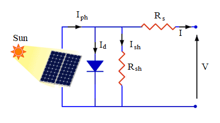
- Single-diode equivalent circuit for PV module [31]
A simplified PV model is used where I is a function of V. The simplified I–V relationship of the PV cell (using the diode equation) is:
| 
| (1) |
where  is the photocurrent (in Amperes),
  is the reverse saturation current of the diode,
  is the thermal voltage and
  is the voltage across the PV cell.
In this study, the following assumptions are adopted to enable a dynamic model of the PV system:
- Constant irradiance: The solar insolation is fixed at 1000 W/m².
- Constant temperature: The cell temperature is assumed constant at 25°C (298 K), removing temperature-dependence from the I-V model.
- Neglecting parasitic effects: Capacitance, recombination losses, and leakage currents beyond
 are excluded.
 - Constant photocurrent (): Taken as 1 A.
- Negligible inductive/capacitive effects: For simplicity, dynamic effects due to reactive elements are ignored.
These assumptions reflect typical standard test conditions (STC) and enable use of the single-diode model for transient analysis. A simplified PV model is chosen as it preserves the nonlinear exponential diode characteristics while reducing model complexity, allowing efficient time-domain simulation of the cell’s dynamic behavior using numerical solvers.
The constants defined for the PV model: in Amperes is = 1 A, Vt in Volts is = 0.025, Shunt resistance in Ohms is =1000 Ohms, Series resistance in Ohms is Rs = 0.02 and Irradiance in W/m2 is G = 1000. This study uses a simplified single-diode PV model under the assumptions of constant irradiance (G = 1000 W/m²), constant temperature (25°C), constant photocurrent ( = 1 A), and negligible dynamic variation in resistive elements. The impact of parasitic capacitance, partial shading, and nonlinear recombination dynamics is excluded for clarity and computational tractability.
Numerical Solvers for PV Models
The basic generalization of the Runge-Kutta-Fehlberg (RKF) method is:
| 
| (2) |
where
where  is a dependent variable,
  is an independent variable, s is a number of stages, bi, ci and aij are coefficients that determined from Butcher tableau [33][34].
The Runge-Kutta-Fehlberg method is widely used, but one of its common applications is the Runge-Kutta-Fehlberg method, also known as the RKF45 method. This method is an algorithm in numerical analysis. The error in solving a given problem according to this method is estimated and controlled using a higher-order integrated method. This method allows the adaptive step size to be determined automatically. The general form of the RKF 45 method is written as follows [35][36]. In [12], ‘Euler method, Runge-Kutta second order, Runge-Kutta fourth order and Runge-Kutta Fehlberg methods’ were presented to solve the initial value problem of ordinary differential equation.
| 
| (6) |
where n=1,2,3, …, and
The error in the solutions can be estimated and controlled by using a higher-order embedded method that allows for an adaptive step size to be determined automatically [12]. MATLAB implementations assess convergence rates and error minimization. Newton's method is widely used for solving nonlinear equations because this type of method is iterative in nature and also has the property of converging quickly [37]. For numerical integration of the nonlinear PV system, the Runge–Kutta–Fehlberg (RKF45) method is employed, providing efficient solutions for complex nonlinear equations [38][39]. The RK4 method is a numerical technique used to solve ordinary differential equations (ODEs). In the context of a PV system, RK4 is used to simulate the behavior of the system, such as its current-voltage characteristics over time under a specific dynamic system, like the dynamics of a MPPT algorithm or energy storage system.
Signal processing can be applied in power systems for better interpretation of voltage signals. For example, wavelet techniques can be used in relation to signal extraction, MPPT enhancement or transient analysis. Wavelet-based signal processing techniques have been used to isolate high-frequency components in PV system voltage or current signals, particularly in the context of MPPT under dynamic environmental conditions. While effective for capturing signal features, these approaches are limited in capturing the system’s underlying nonlinear state evolution, which this paper aims to explore through Lyapunov-based dynamic modeling. Energy feature indicating strength of a signal is used in [40], for extracting useful information from voltage signals. In [41], wavelet-based feature extraction is applied for supply voltage sag monitoring and [42] used wavelet analysis to detect transient faults in PV outputs. The variations in PV voltage can be processed using statistical measures as shown in [43]. AI-based control logic in solar traffic and PV systems is implemented in [44]. Internet of Things (IoT) integration is applied in [45] for PV panels cooling and efficiency enhancement. SVC was used in [46] and this modeling can be used for voltage regulation in PV-connected systems.
In recent years, numerous studies have investigated various techniques to enhance the performance assessment, fault diagnosis, maximum power extraction, and parameter estimation of PV systems. These approaches often rely on data-driven algorithms, hybrid models, and predictive strategies aimed at optimizing PV output under different environmental and operating conditions. A selection of such methods is summarized in the literature, covering power forecasting, soiling analysis, fault detection, and MPPT optimization across diverse platforms and system configurations. A method to accurately find the electrical parameters of PV modules to improve their performance modeling is presented in [47]. A comparison of two control methods is done in [48] to improve the energy output of a 20 kWp solar PV system under different environmental conditions. Ref. [49] focuses on the optimal sizing of standalone PV systems to ensure reliable power supply based on energy needs and solar conditions. It is studied and modelled in [50], the behavior of polycrystalline PV cells for better understanding and prediction of their electrical output. A way to detect performance degradation in solar PV systems by analyzing output uncertainties over time is proposed in [51]. A long-term solar radiation modeling approach has been introduced in [52] to enhance forecasting accuracy and performance planning in PV systems. Performance assessment and degradation detection in grid-connected PV systems have been emphasized in [53] for improving system reliability and maintenance. Detection of PV panel defects has been addressed in [54] through analysis techniques that support timely maintenance and operational stability. A short-term power prediction strategy has been applied in [55] to virtual PV plants to improve dispatch planning and reduce power output uncertainty. Integration of standalone photovoltaic power with desalination systems has been proposed in [56], focusing on energy-efficient control and adaptability.
As dust and dirt gets deposited on PV array, cleaning methods have a significant role in increasing efficiency of PV cells. Soiling-related energy loss in PV systems has been quantified in [57] to aid in developing optimal cleaning strategies for improved performance. Segmentation of PV panels in unevenly illuminated infrared images has been achieved in [58] to support accurate automated inspection. A smart grid energy management framework has been designed in [59] with solar PV integration to balance demand and enhance renewable utilization. Load separation and forecasting in PV-powered smart have been facilitated to support energy optimization strategies in [60]. A one-day-ahead probabilistic forecast of solar power has been enhanced in [61] through imputation techniques for handling incomplete data. A robust PV power generation model tolerant to missing data has been developed in [62] to maintain prediction accuracy under uncertainty. Short-term forecasting of solar PV power has been improved in [63] to better align renewable output with real-time grid demands. Solar PV-based energy harvesting in smart grids has been prioritized in [46] to improve decision-making and optimize system efficiency.
Numerically optimized strategies and approaches can be adapted to photovoltaic systems where precise control and efficiency optimization are essential. It has been suggested in literature that the principles of aerodynamic tuning may be extended to electrical parameter regulation in PV environments to enhance energy conversion under variable operating conditions [64]-[66]. It is demonstrated in [67] that performance optimization using numerical simulation can significantly enhance aerodynamic efficiency, an approach conceptually similar to tracking optimal points in PV systems under variable irradiance using MPPT techniques. It is explained in [68] that numerical and experimental modeling aids in identifying configurations for improved energy capture, drawing parallels to modeling the dynamic I-V curve of a PV cell. It is observed in [69] that design-level optimization can be employed to maximize energy output. Similarly, in PV systems, modifying control algorithms or circuit parameters can lead to improved global power point tracking.
High-frequency ripple extraction in PV system signals has been utilized in [70] to improve the accuracy and performance of MPPT algorithms. A hybrid MPPT strategy was introduced in [71][72] to effectively extract the global maximum power from PV systems under partial shading. Enhanced power output and system performance were achieved by integrating AI with conventional methods. A data-driven architecture was proposed in [73] for diagnosing faults in PV systems based on system health states. Improved accuracy in fault detection and timely maintenance was demonstrated through real-time monitoring. Parameter estimation for photovoltaic systems was conducted in [74] using an advanced optimization approach to improve modeling accuracy. The method contributed to better system characterization and performance prediction. Runge-Kutta method and Lyapunov stability analysis were applied in [2] to study nonlinear dynamics in celestial systems. This methodology is similarly used in this work to analyze the nonlinear voltage-current behavior and stability of PV cells.
While these works significantly contribute to performance modeling and control, they typically focus on algorithmic implementation rather than providing deep insights into the nonlinear dynamical behavior of PV cells. To address this gap, the present study employs Lyapunov stability theory in conjunction with RK4 integration to perform a dynamic analysis of PV cell behavior under varying irradiance and load conditions. This mathematical approach enables a robust time-domain investigation of the PV system’s response characteristics, offering a complementary perspective to existing data-driven and optimization-based models.
Fourth-Order Runge-Kutta Simulation of a PV System
The simulation models the dynamic behavior of a PV cell over time using the RK4 method. RK4 is a powerful numerical integration technique used to solve ordinary differential equations (ODEs) with high accuracy. In this context, it is used to compute how the voltage and current of a PV cell evolve over time based on a nonlinear differential equation derived from the PV model. The PV system is modelled based on the single-diode equivalent circuit, which describes the relationship between the output current and voltage of a solar cell. The key parameters used in the simulation include [75]:
- Photocurrent : The current generated by the solar irradiance.
- Reverse saturation current : The leakage current of the diode in reverse bias.
- Thermal voltage : Given by
 where
where  is Boltzmann’s constant,
  is absolute temperature, and
  is the electron charge.
 - Series resistance
 : Represents internal resistance losses.
 - Shunt resistance : Models leakage paths within the cell.
Numerical Setup for RK4 is given by:
- Time step:
 = 0.01 seconds
 - Total simulation time: 5 seconds
- Initial condition: V (0) = 0
- Number of iterations: 500
- Key constants: = 1A;
 = 10-6A; = 0.025 V; = 0.02 Ω and = 1000 Ω
This fixed-step simulation ensures uniform sampling for Lyapunov analysis and visualization.
The current in the PV cell, ignoring and for simplification, can be expressed as:
| 
| (13) |
To simulate the voltage over time, a first-order differential form is assumed:
| 
| (14) |
Equation (14) represents the dynamic voltage evolution as a first-order nonlinear ODE. This is derived by assuming constant and neglecting the effect of and temporarily, isolating the system’s voltage-driven dynamic response. This is a nonlinear ODE, which is solved using RK4. RK4 estimates the future value of a variable by taking a weighted average of four increments (slopes). The dynamic model given by Equation 14 is a simplification derived from the single-diode equivalent circuit. This approximation, while neglecting certain nonlinearities, retains the essential features of the exponential diode response and is validated by convergence behavior [76]-[78]. Let  be the voltage at time
  ,
,  be the time step. The update rule is:
After updating the voltage, the corresponding current is calculated using the PV equation. Table 1 and Table 2 details algorithm descriptions for RK4 and RKF45 adaptive step Integration for PV Cell Voltage Simulation.
Table 1. RK4 Integration for PV Cell Voltage Simulation
S. No | Step | Description |
1 | Initialize parameters | Define all necessary constants such as photocurrent (), reverse saturation current (), thermal voltage (), series resistance (), and time step (). |
2 | Define initial condition | Set the starting voltage (0) = 0. |
3 | Define the current-voltage function | This function models how the current behaves for a given voltage. Use:
 |
4 | Use the RK4 method to compute intermediate values | For each time step n, calculate: |

|

|

|

|
5 | Update the voltage | Use RK4 formula: |
|
| 
|
6 | Update the current | Recalculate the current using the updated voltage. |
7 | Repeat the process | Continue the loop for all time steps to simulate the system response. |
8 | Store and plot results | Store voltage and current values and generate time-domain plots. |
The following are considered for simulation setup:
- Initial Conditions: The voltage starts at zero, and the corresponding initial current is computed.
- Time Range: The simulation runs from
 to
to  second with a step size
  0.01 seconds.
 - Arrays for voltage
 and current
  are initialized and updated at each time step using the RK4 method.
The following simplifications provide a first-order nonlinear model that can be solved numerically: Constant , Negligible series resistance for ODE formulation, No load variation and no MPPT perturbation.
Table 2. RKF45 Integration for PV Cell Voltage Simulation
S. No | Step | Description |
1 | Define the voltage-current relationship | Use the same function as in Algorithm 1. |
2 | Set simulation start and end time | Choose time span (e.g., 0 to 5 s) and initial voltage (e.g., 0 V). |
3 | Select error tolerance | Choose a small value like 0.001 to control step size adaptively. |
4 | Compute two estimates | RKF45 calculates 4th and 5th-order estimates of voltage per step. |
5 | Calculate error | Estimate the error by comparing both voltage approximations. |
6 | Adjust step size | Increase step size if error is small, or decrease if too large. |
7 | Accept or reject step | Accept results if error is within tolerance; otherwise, recompute. |
8 | Repeat steps | Continue until reaching the end of simulation. |
9 | Store and analyze output | Store and plot voltage and current data to visualize response. |
The RK4 method effectively simulates the nonlinear dynamic behavior of a PV cell. By solving the governing equation iteratively, it is observed how voltage and current evolve in response to constant irradiance. The resulting plots are essential to understand both the charging behavior and stability characteristics of PV systems over time. Table 3 shows comparison between RK4 and RKF45 for different parameters and Figure 2 shows different features of both these methods. In this paper, RK4 is used for deterministic output and RKF45 is referenced and not implemented. This study uses RK4 for its deterministic behavior, aligning well with fixed sampling for Lyapunov stability analysis. RK4 is used as this method offers a good trade-off between computational load and accuracy. Its fixed-step nature ensures consistent sampling, ideal for derivative-based stability analysis such as Lyapunov methods. Interpretation of plots is depicted in Figure 3.
Table 3. Comparison between RK4 and RKF45 methods
Method | Step Size | Error Estimation | Use Case | Complexity |
RK4 | Fixed | None | Simple systems | Low |
RKF45 (ode45) | Adaptive | Built-in | Systems needing error control | Moderate |
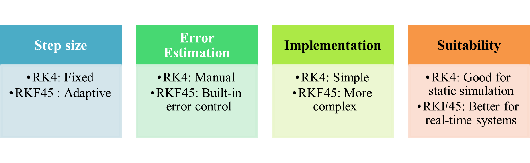
- Different features of RK4 and RKF45 methods
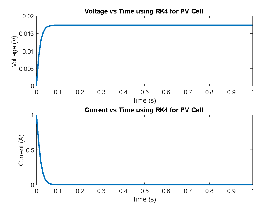
- Variation of Voltage over time and Current over time
Voltage vs. Time Plot
- This plot in Figure 3 shows how the voltage across the PV cell evolves over time.
- The curve typically increases smoothly as the system responds to a constant illumination, eventually stabilizing.
- The shape depends on how the exponential diode behavior influences the voltage growth.
Current vs. Time Plot
- This plot in Figure 3 illustrates the change in output current over time.
- Since the photocurrent is constant, and the diode current increases with voltage, the net current decreases slightly or stabilizes, depending on the dynamics.
- The plot helps observe the transient behavior before reaching steady-state.
The RK4 method approximates the solution to an ODE by evaluating the differential equation at multiple points in each time step and computing the weighted average of these values.
The update rule is:
| 
| (20) |
where  are the intermediate slopes calculated at each time step. The voltage and current are updated at each time step using the RK4 method, and the voltage-current relationship is updated accordingly. The results show the voltage and current variations over time. These plots shown in Figure 3 provide insight into how the PV system behaves dynamically over time. Key assumptions:
- The dynamics of the PV system are modelled using a simple current-voltage relationship.
- The code doesn’t account for more complex factors such as temperature variation, partial shading, or detailed MPPT algorithms.
- The RK4 method is applied to solve the system over a discrete time grid.
Lyapunov-Based Stability Assessment for PV Systems
Having modelled the system dynamics using RK4, the system’s intrinsic stability characteristics through Lyapunov analysis is examined, which complements the numerical simulation by providing a theoretical guarantee of convergence. Stability is assessed by computing Lyapunov exponents for PV system dynamics. These metrics quantify system divergence from equilibrium under varying irradiance and load conditions. A refined Lyapunov-based function is introduced for real-time MPPT optimization. The Lyapunov function used is a quadratic energy-based formulation, which is a classical candidate Lyapunov function for scalar systems, measuring the deviation of the current from its equilibrium value. It allows analysis of the system’s potential to return to a steady-state following perturbation. Lyapunov analysis offers a formal mechanism to verify that system trajectories converge to a stable equilibrium. This is especially relevant for PV systems, where unpredictable irradiance or load changes may affect power output. Lyapunov-based methods are foundational for nonlinear control and stability assessment. Their application in PV ensures that, even under small perturbations, the system will not exhibit oscillations or instability—crucial for grid-connected applications and MPPT. Despite the presence of adaptive RKF45, the fixed-step RK4 was used to ensure consistent sampling intervals, necessary for accurate Lyapunov derivative approximation and phase plot generation.
The PV system converts light into electrical power. The current generated by the PV system can be modelled as a function of the voltage. The simplified I-V equation for a PV cell [79][80]:
| 
| (21) |
where  is the output current of the PV cell (A), is the photocurrent (A), which is directly proportional to the irradiance (G), is the reverse saturation current of the diode (A), representing a small leakage current, is the thermal voltage (V), defined as
  with
with  being Boltzmann’s constant,
  the temperature in Kelvin, and the charge of an electron, is the terminal voltage (V), is the series resistance (Ω), modeling the internal resistance in series with the output.
In stability analysis, the Lyapunov function  is used to evaluate the stability of the PV system. The Lyapunov function is a scalar function that measures the ‘energy-like’ quantity of the system. ‘Energy-like’ in this context means the Lyapunov function behaves analogously to a physical energy measure—it is always positive and decreases over time, indicating dissipation and convergence toward equilibrium. If the derivative of the Lyapunov function is negative, the system is stable and tends to return to equilibrium. The Lyapunov function is given by:
| 
| (22) |
where  is the instantaneous current and
  is the equilibrium current. At equilibrium,
  .
.
The equilibrium current  is the value of when the voltage
  , which can be calculated as:
| 
| (23) |
The derivative of the Lyapunov function  is used to assess the system’s stability. If the derivative is negative
  , the system is stable and will return to equilibrium. The time derivative of the Lyapunov function is:
| 
| (24) |
To calculate  , we differentiate the current with respect to time (or voltage). The expression for the derivative of current is approximated as:
| 
| (25) |
where  represents the change in current with respect to the change in voltage, derived from the diode’s exponential current-voltage relation. The stability of the system is analyzed by examining the sign of the time derivative of the Lyapunov function, If
  for all values of , the system is stable, and the PV system will return to its equilibrium state, If
  , the system is unstable, and the current may diverge from equilibrium, If
  , the system is marginally stable.
The Lyapunov function provides a powerful tool for analyzing the stability of dynamic systems. In the context of the PV system, it helps determine whether the system will stabilize at an equilibrium point or if it may diverge under certain conditions. By analyzing the Lyapunov function and its derivative, we can conclude that the PV system will remain stable as long as remains negative for all voltages. To perform Lyapunov stability analysis for a PV (PV) system, we generally analyze the stability of the system by deriving a Lyapunov function and evaluating its derivative over time. This is typically done for dynamic systems such as the MPPT controller for PV systems. A basic PV system (using a simple model) is simulated, a Lyapunov function is defined and the results of the stability analysis are plotted as shown in Figure 4.
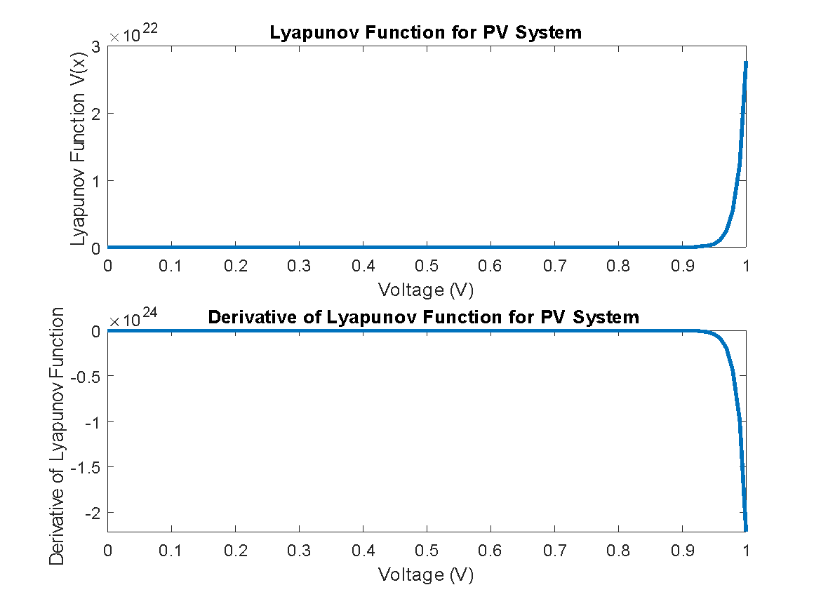
- Lyapunov function plot and derivative of Lyapunov function plot
Figure 4 shows the Lyapunov function over the range of voltage and the time derivative of the Lyapunov function, which gives insight into the stability of the system. A simplified PV model is considered and does not include more detailed effects such as temperature variation, shading, or nonlinearities in the current-voltage characteristics. Lyapunov stability analysis assumes a well-defined equilibrium point and checks if the system will return to equilibrium after a disturbance. The derivative of the Lyapunov function should ideally be negative for all states (except the equilibrium), which implies stability. Lyapunov stability analysis is crucial in PV system modeling as it assesses whether the system will return to an equilibrium operating point after a small disturbance. This ensures reliable energy output and supports the development of robust MPPT algorithms. Without such stability, PV systems may oscillate or respond unpredictably to environmental variation. Table 4 gives algorithm for Lyapunov Stability Analysis of PV System.
Table 4. Algorithm for Lyapunov Stability Analysis of PV System
S. No | Step | Description |
1 | Define the system's equilibrium current | Take the final or steady-state current value from the simulation, denoted as . |
2 | Define the Lyapunov function | Use:  This measures the deviation from equilibrium. This measures the deviation from equilibrium. |
3 | Compute the derivative of the Lyapunov function | Use finite difference:  |
4 | Analyze the sign of the derivative | If  , the system is stable; if > 0, it may be unstable. , the system is stable; if > 0, it may be unstable. |
5 | Visualize the results | Plot V(t) and over time. A decreasing V(t) indicates stability. |
6 | Interpret the outcome | If V(t) decreases and is negative, the PV system returns to equilibrium, confirming stability. |
Interpretation of Simulation Results
The obtained simulation results are interpreted as below:
- Voltage increases nonlinearly and stabilizes, reflecting diode saturation.
- Current decreases slightly due to increasing diode conduction.
- Stabilization time ≈ 1–1.5 seconds.
- Voltage Response: Voltage rises smoothly and settles at a constant level, indicating proper diode behavior and system convergence.
- Current Response: Current shows transient decay, settling as diode saturation effects dominate.
- System Stability: The system reaches a steady state in under 1 second, suggesting rapid dynamic stabilization.
- Design Implication: Stability confirms the reliability of using fixed-parameter models for real-time simulations.
- This confirms proper time response and non-oscillatory behavior.
The main finding of this study is that a simplified PV model, when analyzed using the RK4 numerical integration technique, exhibits stable dynamic behavior under constant irradiance. The Lyapunov function further confirms this stability by consistently yielding a negative derivative over time, implying convergence to equilibrium. Compared with traditional steady-state I-V curve methods, our approach captures transient behavior critical for the design of real-time MPPT controllers. Other studies have focused primarily on static conditions or open-loop responses, whereas our work links numerical integration with theoretical energy-based stability. These findings imply that such simplified yet dynamic models can serve as foundational tools for AI-based PV control and optimization systems.
The use of RK4 ensures reproducibility and low computational complexity, while Lyapunov functions offer analytical assurance of performance. Strengths include: the hybrid use of RK4 and Lyapunov analysis, clarity of dynamic response, and practical adaptability. Limitations include: constant irradiance and temperature, absence of external control (e.g., MPPT), and use of a reduced-order model which may not capture all real-world nonlinearities. Voltage stabilizes smoothly, while the output current converges with minor transients. These behaviors confirm the dynamic equilibrium nature of the system under constant irradiance. The combination of RK4 numerical simulation and Lyapunov energy-based stability analysis provides a unified approach, filling a gap in PV modeling literature that typically addresses either numerical or theoretical methods in isolation.
MODEL VALIDITY AND REAL-TIME RELEVANCE
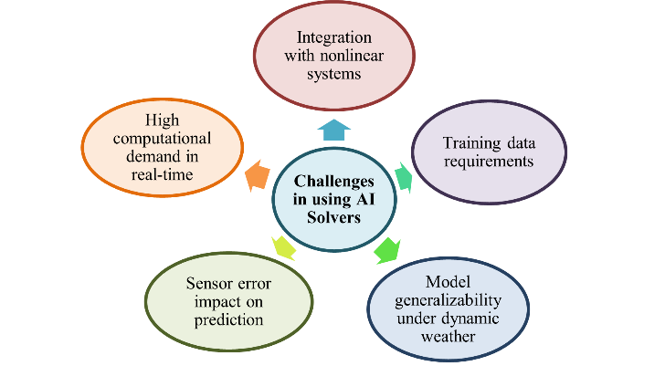
Although a simplified single-diode model is used in this study by assuming constant temperature, ideal diode behavior, and negligible series/shunt resistances, such assumptions do not hold in practical PV systems operating under real-time conditions. In real environments, factors such as fluctuating irradiance, temperature variations, and aging of PV modules introduce dynamic nonlinearities. To bridge this gap, real-time parameter estimation techniques are often employed to continuously update the model with accurate system data. Additionally, wavelet analysis can be integrated to decompose voltage or current signals into frequency components, allowing the identification of transients, shading effects, or electrical faults. With these enhancements, the nonlinear stability analysis using Lyapunov functions and the time-domain simulation via RK4 integration remain applicable, offering insights into the system's dynamic behavior under realistic operational disturbances. The current model sets the foundation for AI integration, where machine learning algorithms could adapt control parameters in real time, enhancing MPPT under rapidly changing conditions. Figure 5 illustrates few general challenges faced in using AI solvers which are to be addressed effectively by researchers. The study confirms that RK4 captures transient dynamics effectively. Compared to static PV models, this method offers greater insight into system response. Lyapunov analysis complements it by formally confirming system stability. While strong in simplicity and reproducibility, limitations include constant environmental conditions and the absence of MPPT logic. Future work will explore AI-based adaptation and model validation under real-time solar data.

- Challenges in using AI solvers
- CONCLUSIONS
The integration of RK4 numerical simulation and Lyapunov stability analysis provides a comprehensive understanding of a PV cell's dynamic behavior under constant irradiance. The simulation results confirm that the PV cell reaches a stable operating point over time, as evidenced by the Lyapunov function's decreasing trend. This study underscores the effectiveness of combining numerical and analytical methods for analyzing and ensuring the stability of PV systems. Simulation validates the dynamic behavior and confirms stability through negative Lyapunov derivatives. Future research will focus on the integration of real-time AI-driven numerical solvers to further enhance MPPT performance and improve grid stability. Machine learning algorithms combined with numerical solvers can provide adaptive control strategies that respond more efficiently to fluctuating irradiance and load conditions. Such advancements will drive the next generation of intelligent, self-optimizing PV systems for large-scale renewable energy integration. The PV system shows stable behavior under constant irradiance when analyzed via RK4 integration and Lyapunov functions. The simulation results validate the reliability of using this simplified dynamic model for further control or optimization studies.
DECLARATION
Author Contribution
All authors contributed equally to the main contributor to this paper. All authors read and approved the final paper.
Funding
This research received no external funding.
Conflicts of Interest
The authors declare no conflict of interest.
REFERENCES
- K. Mohamed, H. Shareef, I. Nizam, A. B. Esan, and A. Shareef, “Operational Performance Assessment of Rooftop PV Systems in the Maldives,” Energy Reports, vol. 11, pp. 2592–2607, 2024, https://doi.org/10.1016/j.egyr.2024.02.014.
- A. Hysa, M. M. Mahmoud, and A. Ewais, “An Investigation of the Output Characteristics of Photovoltaic Cells Using Iterative Techniques and MATLAB ® 2024a Software,” Control Syst. Optim. Lett., vol. 3, no. 1, pp. 46–52, 2025, https://doi.org/10.59247/csol.v3i1.174.
- M. Awad et al., “A review of water electrolysis for green hydrogen generation considering PV/wind/hybrid/hydropower/geothermal/tidal and wave/biogas energy systems, economic analysis, and its application,” Alexandria Eng. J., vol. 87, pp. 213–239, 2024, https://doi.org/10.1016/j.aej.2023.12.032.
- A. Hysa And M. Klemo, “Modeling and Simulation of Photovioltaic Cell With Matlab for Different Temperature and Different Solar Radiation,” Interdiscip. J. Res. Dev., vol. 6, no. 2, p. 44, 2019, https://doi.org/10.56345/ijrdv6n204.
- X. H. Nguyen and M. P. Nguyen, “Mathematical modeling of photovoltaic cell/module/arrays with tags in Matlab/Simulink,” Environ. Syst. Res., vol. 4, no. 1, 2015, https://doi.org/10.1186/s40068-015-0047-9.
- M. Metwally Mahmoud, “Improved current control loops in wind side converter with the support of wild horse optimizer for enhancing the dynamic performance of PMSG-based wind generation system,” Int. J. Model. Simul., vol. 43, no. 6, pp. 952–966, 2023, https://doi.org/10.1080/02286203.2022.2139128.
- E. Karatepe, M. Boztepe, and M. Colak, “Neural network based solar cell model,” Energy Convers. Manag., vol. 47, no. 9–10, pp. 1159–1178, 2006, https://doi.org/10.1016/j.enconman.2005.07.007.
- M. Battaglia, E. Comi, T. Stadelmann, R. Hiestand, B. Ruhstaller, and E. Knapp, “Deep ensemble inverse model for image-based estimation of solar cell parameters,” APL Mach. Learn., vol. 1, no. 3, 2023, https://doi.org/10.1063/5.0139707.
- M. M. Mahmoud et al., “Application of Whale Optimization Algorithm Based FOPI Controllers for STATCOM and UPQC to Mitigate Harmonics and Voltage Instability in Modern Distribution Power Grids,” Axioms, vol. 12, no. 5, 2023, https://doi.org/10.3390/axioms12050420.
- A. Mousa, “Maximum Power Point Tracking Achievements and Challenges in Photovoltaic Systems,” Brill. Res. Artif. Intell., vol. 3, no. 2, pp. 68–80, 2023, https://doi.org/10.47709/brilliance.v3i2.2385.
- A. Hysa, “Modeling and simulation of the photovoltaic cells for different values of physical and environmental parameters,” Emerg. Sci. J., vol. 3, no. 6, pp. 395–406, 2019, https://doi.org/10.28991/esj-2019-01202.
- M. M. M. Azem Hysa, M.S. Priyadarshini, “Numerical Solution of the System of Non-Linear Differential Equations of the Three-Body Problem in a Special Case,” Eur. Mod. Stud. J., vol. 9, no. 1, pp. 42–56, 2025, https://doi.org/10.59573/emsj.9(1).2025.6.
- G. G. Rigatos, M. Abbaszadeh, B. Sari, and J. Pomares, “Nonlinear optimal control for UAVs with tilting rotors,” Int. J. Intell. Unmanned Syst., vol. 12, no. 1, pp. 32–104, 2024, https://doi.org/10.1108/IJIUS-02-2023-0018.
- K. Tifidat, N. Maouhoub, A. Benahmida, and F. Ezzahra Ait Salah, “An accurate approach for modeling I-V characteristics of photovoltaic generators based on the two-diode model,” Energy Convers. Manag. X, vol. 14, 2022, https://doi.org/10.1016/j.ecmx.2022.100205.
- I. K. Argyros, “Concerning the convergence of Newton’s method and quadratic majorants,” J. Appl. Math. Comput., vol. 29, no. 1–2, pp. 391–400, 2009, https://doi.org/10.1007/s12190-008-0140-6.
- B. T. Polyak, “Newton’s method and its use in optimization,” Eur. J. Oper. Res., vol. 181, no. 3, pp. 1086–1096, 2007, https://doi.org/10.1016/j.ejor.2005.06.076.
- O. M. Kamel, A. A. Z. Diab, M. M. Mahmoud, A. S. Al-Sumaiti, and H. M. Sultan, “Performance Enhancement of an Islanded Microgrid with the Support of Electrical Vehicle and STATCOM Systems,” Energies, vol. 16, no. 4, 2023, https://doi.org/10.3390/en16041577.
- D. Cherifi, M. Boudjada, A. Morsli, G. Girard, and R. Deriche, “Combining Improved Euler and Runge-Kutta 4th order for Tractography in Diffusion-Weighted MRI,” Biomed. Signal Process. Control, vol. 41, pp. 90–99, 2018, https://doi.org/10.1016/j.bspc.2017.11.008.
- Z. Usman, J. Tah, H. Abanda, and C. Nche, “A critical appraisal of pv‐systems’ performance,” Buildings, vol. 10, no. 11. pp. 1–23, 2020, https://doi.org/10.3390/buildings10110192.
- I. Inderjeet and R. Bhardwaj, “Numerical Simulation of Ordinary Differential Equation by Euler and Runge–Kutta Technique,” J. Electron. Netw. Appl. Math., no. 36, pp. 8–17, 2023, https://doi.org/10.55529/jecnam.36.8.17.
- M. Adel and M. M. Khader, “Theoretical and numerical treatment for the fractal-fractional model of pollution for a system of lakes using an efficient numerical technique,” Alexandria Eng. J., vol. 82, pp. 415–425, 2023, https://doi.org/10.1016/j.aej.2023.10.003.
- J. C. Domínguez et al., “MATLAB applications for teaching Applied Thermodynamics: Thermodynamic cycles,” Comput. Appl. Eng. Educ., vol. 31, no. 4, pp. 900–915, 2023, https://doi.org/10.1002/cae.22613.
- M. S. Priyadarshini, D. Krishna, M. B. Reddy, A. Bhatt, M. Bajaj and M. M. Mahmoud, "Continuous Wavelet Transform based Visualization of Transient and Short Duration Voltage Variations," 2023 4th IEEE Global Conference for Advancement in Technology (GCAT), pp. 1-6, 2023, https://doi.org/10.1109/GCAT59970.2023.10353457.
- R. Engelken, F. Wolf, and L. F. Abbott, “Lyapunov spectra of chaotic recurrent neural networks,” Phys. Rev. Res., vol. 5, no. 4, 2023, https://doi.org/10.1103/PhysRevResearch.5.043044.
- P. S. Madur, S. Malaji, and R. Kuruva, “Wavelet transform based statistical feature extraction of power quality disturbances,” in AIP Conference Proceedings, vol. 2755, no. 1, 2023, https://doi.org/10.1063/5.0148333.
- S. Heroual, B. Belabbas, and N. B. Elzein I M, Yasser Diab, Alfian Ma’arif, Mohamed Metwally Mahmoud, Tayeb Allaoui, “Enhancement of Transient Stability and Power Quality in Grid- Connected PV Systems Using SMES,” Int. J. Robot. Control Syst., vol. 5, no. 2, pp. 990–1005, 2025, https://doi.org/10.31763/ijrcs.v5i2.1760.
- H. Boudjemai et al., “Design, Simulation, and Experimental Validation of a New Fuzzy Logic-Based Maximal Power Point Tracking Strategy for Low Power Wind Turbines,” Int. J. Fuzzy Syst., vol. 5, no. 1, pp. 296–310, 2025, https://doi.org/10.31763/ijrcs.v5i1.1425.
- O. M. Lamine et al., “A Combination of INC and Fuzzy Logic-Based Variable Step Size for Enhancing MPPT of PV Systems,” Int. J. Robot. Control Syst., vol. 4, no. 2, pp. 877–892, 2024, https://doi.org/10.31763/ijrcs.v4i2.1428.
- I. El Maysse et al., “Nonlinear Observer-Based Controller Design for VSC-Based HVDC Transmission Systems Under Uncertainties,” IEEE Access, vol. 11, pp. 124014–124030, 2023, https://doi.org/10.1109/ACCESS.2023.3330440.
- M. S. Priyadarshini, A. Sravani, S. Gochhait, A. Bhatt, M. Bajaj and M. M. Mahmoud, "IoT Platform-Based Prototype Model of an Adaptive and Intelligent Traffic Lighting System," 2023 4th IEEE Global Conference for Advancement in Technology (GCAT), pp. 1-6, , 2023. https://doi.org/10.1109/GCAT59970.2023.10353407.
- N. F. Ibrahim et al., “Operation of Grid-Connected PV System with ANN-Based MPPT and an Optimized LCL Filter Using GRG Algorithm for Enhanced Power Quality,” IEEE Access, vol. 11, pp. 106859–106876, 2023, https://doi.org/10.1109/ACCESS.2023.3317980.
- N. F. Ibrahim et al., “A new adaptive MPPT technique using an improved INC algorithm supported by fuzzy self-tuning controller for a grid-linked photovoltaic system,” PLoS One, vol. 18, pp. 1–22, 2023, https://doi.org/10.1371/journal.pone.0293613.
- M. S. Priyadarshini and M. Sushama, “Performance of Static VAR Compensator for Changes in Voltage Due to Sag and Swell,” in Lecture Notes in Electrical Engineering, pp. 225–233, 2020, https://doi.org/10.1007/978-981-15-2256-7_22.
- H. Zhang, A. A. Heidari, M. Wang, L. Zhang, H. Chen, and C. Li, “Orthogonal Nelder-Mead moth flame method for parameters identification of photovoltaic modules,” Energy Convers. Manag., vol. 211, 2020, https://doi.org/10.1016/j.enconman.2020.112764.
- P. C. Babu, B. V. Prasanth, and P. Sujatha, “Implementation of anfis-mptc for 20 kwp spv power generation and comparison with flmppt under dissimilar conditions,” Int. J. Ambient Energy, vol. 43, no. 1, pp. 1445–1455, 2022, https://doi.org/10.1080/01430750.2019.1707117.
- B. Cortés, R. Tapia Sánchez, and J. J. Flores, “Characterization of a polycrystalline photovoltaic cell using artificial neural networks,” Sol. Energy, vol. 196, pp. 157–167, 2020, https://doi.org/10.1016/j.solener.2019.12.012.
- M. Alrifaey et al., “Hybrid Deep Learning Model for Fault Detection and Classification of Grid-Connected Photovoltaic System,” IEEE Access, vol. 10, pp. 13852–13869, 2022, https://doi.org/10.1109/ACCESS.2022.3140287.
- L. Li, Z. Wang, and T. Zhang, “GBH-YOLOv5: Ghost Convolution with BottleneckCSP and Tiny Target Prediction Head Incorporating YOLOv5 for PV Panel Defect Detection,” Electron., vol. 12, no. 3, 2023, https://doi.org/10.3390/electronics12030561.
- X. Zhou, C. Pang, X. Zeng, L. Jiang, and Y. Chen, “A Short-Term Power Prediction Method Based on Temporal Convolutional Network in Virtual Power Plant Photovoltaic System,” IEEE Trans. Instrum. Meas., vol. 72, 2023, https://doi.org/10.1109/TIM.2023.3301904.
- H. D. Nejad et al., “Fuzzy State-Dependent Riccati Equation (FSDRE) Control of the Reverse Osmosis Desalination System With Photovoltaic Power Supply,” IEEE Access, vol. 10, pp. 95585–95603, 2022, https://doi.org/10.1109/ACCESS.2022.3204270.
- W. Zhang, S. Liu, O. Gandhi, C. D. Rodriguez-Gallegos, H. Quan, and D. Srinivasan, “Deep-learning-based probabilistic estimation of solar PV soiling loss,” IEEE Trans. Sustain. Energy, vol. 12, no. 4, pp. 2436–2444, 2021, https://doi.org/10.1109/TSTE.2021.3098677.
- N. Wang, Z. L. Sun, Z. Zeng, and K. M. Lam, “Effective Segmentation Approach for Solar Photovoltaic Panels in Uneven Illuminated Color Infrared Images,” IEEE J. Photovoltaics, vol. 11, no. 2, pp. 478–484, 2021, https://doi.org/10.1109/JPHOTOV.2020.3041189.
- A. Kumar, M. Alaraj, M. Rizwan, and U. Nangia, “Novel AI Based Energy Management System for Smart Grid with RES Integration,” IEEE Access, vol. 9, pp. 162530–162542, 2021, https://doi.org/10.1109/ACCESS.2021.3131502.
- R. E. Alden, H. Gong, E. S. Jones, C. Ababei, and D. M. Ionel, “Artificial Intelligence Method for the Forecast and Separation of Total and HVAC Loads with Application to Energy Management of Smart and NZE Homes,” IEEE Access, vol. 9, pp. 160497–160509, 2021, https://doi.org/10.1109/ACCESS.2021.3129172.
- Q. T. Phan, Y. K. Wu, and Q. D. Phan, “Enhancing One-Day-Ahead Probabilistic Solar Power Forecast With a Hybrid Transformer-LUBE Model and Missing Data Imputation,” IEEE Trans. Ind. Appl., vol. 60, no. 1, pp. 1396–1408, 2024, https://doi.org/10.1109/TIA.2023.3325798.
- Q. Li, Y. Xu, B. S. H. Chew, H. Ding, and G. Zhao, “An Integrated Missing-Data Tolerant Model for Probabilistic PV Power Generation Forecasting,” IEEE Trans. Power Syst., vol. 37, no. 6, pp. 4447–4459, 2022, https://doi.org/10.1109/TPWRS.2022.3146982.
- Y. Cai et al., “Short-Term Power Prediction by Using Least Square Support Vector Machine With Variational Mode Decomposition in a Photovoltaic System,” IEEE Access, vol. 11, pp. 143486–143500, 2023, https://doi.org/10.1109/ACCESS.2023.3343103.
- R. K. Patel, A. Kumari, S. Tanwar, W. C. Hong, and R. Sharma, “AI-Empowered Recommender System for Renewable Energy Harvesting in Smart Grid System,” IEEE Access, vol. 10, pp. 24316–24326, 2022, https://doi.org/10.1109/ACCESS.2022.3152528.
- H. Seifi Davari, S. Kouravand, M. Seify Davari, and Z. Kamalnejad, “Numerical investigation and aerodynamic simulation of Darrieus H-rotor wind turbine at low Reynolds numbers,” Energy Sources, Part A Recover. Util. Environ. Eff., vol. 45, no. 3, pp. 6813–6833, 2023, https://doi.org/10.1080/15567036.2023.2213670.
- T. Shi, G. Hu, and L. Zou, “Aerodynamic Shape Optimization of an Arc-Plate-Shaped Bluff Body via Surrogate Modeling for Wind Energy Harvesting,” Appl. Sci., vol. 12, no. 8, 2022, https://doi.org/10.3390/app12083965.
- M. Pokharel, A. Ghosh, and C. N. M. Ho, “Small-Signal Modelling and Design Validation of PV-Controllers with INC-MPPT Using CHIL,” IEEE Trans. Energy Convers., vol. 34, no. 1, pp. 361–371, 2019, https://doi.org/10.1109/TEC.2018.2874563.
- A. Pramanik, H. Singh, R. Chandra, V. K. Vijay, and S. Suresh, “Amorphous carbon based nanofluids for direct radiative absorption in solar thermal concentrators – Experimental and computational study,” Renew. Energy, vol. 183, pp. 651–661, 2022, https://doi.org/10.1016/j.renene.2021.11.047.
- M. Z. El Masry, A. Mohammed, F. Amer, and R. Mubarak, “New Hybrid MPPT Technique Including Artificial Intelligence and Traditional Techniques for Extracting the Global Maximum Power from Partially Shaded PV Systems,” Sustain., vol. 15, no. 14, 2023, https://doi.org/10.3390/su151410884.
- A. Abubakar, C. F. M. Almeida, and M. Gemignani, “Review of artificial intelligence-based failure detection and diagnosis methods for solar photovoltaic systems,” Machines, vol. 9, no. 12. 2021, https://doi.org/10.3390/machines9120328.
- L. Liang, T. Su, Y. Gao, F. Qin, and M. Pan, “FCDT-IWBOA-LSSVR: An innovative hybrid machine learning approach for efficient prediction of short-to-mid-term photovoltaic generation,” J. Clean. Prod., vol. 385, 2023 https://doi.org/10.1016/j.jclepro.2022.135716.
- M. Colak and S. Balci, “Photovoltaic System Parameter Estimation Using Marine Predators Optimization Algorithm Based on Multilayer Perceptron,” Electr. Power Components Syst., vol. 50, no. 18, pp. 1087–1099, 2022, https://doi.org/10.1080/15325008.2022.2146234.
- N. F. Ibrahim, A. Alkuhayli, A. Beroual, U. Khaled, and M. M. Mahmoud, “Enhancing the Functionality of a Grid-Connected Photovoltaic System in a Distant Egyptian Region Using an Optimized Dynamic Voltage Restorer: Application of Artificial Rabbits Optimization,” Sensors, vol. 23, no. 16, 2023, https://doi.org/10.3390/s23167146.
- A. H. Elmetwaly et al., “Modeling, Simulation, and Experimental Validation of a Novel MPPT for Hybrid Renewable Sources Integrated with UPQC: An Application of Jellyfish Search Optimizer,” Sustain., vol. 15, no. 6, 2023, https://doi.org/10.3390/su15065209.
- N. F. Ibrahim et al., “Multiport Converter Utility Interface with a High-Frequency Link for Interfacing Clean Energy Sources (PV\Wind\Fuel Cell) and Battery to the Power System: Application of the HHA Algorithm,” Sustainability, vol. 15, no. 18, p. 13716, 2023, https://doi.org/10.3390/su151813716.
- M. Awad, M. M. Mahmoud, Z. M. S. Elbarbary, L. Mohamed Ali, S. N. Fahmy, and A. I. Omar, “Design and analysis of photovoltaic/wind operations at MPPT for hydrogen production using a PEM electrolyzer: Towards innovations in green technology,” PLoS One, vol. 18, no. 7, p. e0287772, 2023, https://doi.org/10.1371/journal.pone.0287772.
- R. Kassem et al., “A Techno-Economic-Environmental Feasibility Study of Residential Solar Photovoltaic / Biomass Power Generation for Rural Electrification : A Real Case Study,” Sustain., vol. 16, no. 5, p. 2036, 2024, doi: https://doi.org/10.3390/su16052036.
- A. M. Ewais, A. M. Elnoby, T. H. Mohamed, M. M. Mahmoud, Y. Qudaih, and A. M. Hassan, “Adaptive frequency control in smart microgrid using controlled loads supported by real-time implementation,” PLoS One, vol. 18, no. 4, p. e0283561, 2023, https://doi.org/10.1371/journal.pone.0283561.
- S. R. K. Joga et al., “Applications of tunable-Q factor wavelet transform and AdaBoost classier for identification of high impedance faults: Towards the reliability of electrical distribution systems,” Energy Explor. Exploit., vol. 42, no. 6, pp. 2017-2055, 2024, https://doi.org/10.1177/01445987241260949.
- H. Boudjemai et al., “Experimental Analysis of a New Low Power Wind Turbine Emulator Using a DC Machine and Advanced Method for Maximum Wind Power Capture,” IEEE Access, vol. PP, p. 1, 2023, https://doi.org/10.1109/ACCESS.2023.3308040.
- M. M. Mahmoud, B. S. Atia, A. Y. Abdelaziz, and N. A. N. Aldin, “Dynamic Performance Assessment of PMSG and DFIG-Based WECS with the Support of Manta Ray Foraging Optimizer Considering MPPT, Pitch Control, and FRT Capability Issues,” Processes, vol. 10, no. 12, 2022, https://doi.org/10.3390/pr10122723.
- H. Boudjemai et al., “Application of a Novel Synergetic Control for Optimal Power Extraction of a Small-Scale Wind Generation System with Variable Loads and Wind Speeds,” Symmetry (Basel)., vol. 15, no. 2, 2023, https://doi.org/10.3390/sym15020369.
- S. A. Mohamed, N. Anwer, and M. M. Mahmoud, “Solving optimal power flow problem for IEEE-30 bus system using a developed particle swarm optimization method: towards fuel cost minimization,” Int. J. Model. Simul., vol. 00, no. 00, pp. 1–14, 2023, https://doi.org/10.1080/02286203.2023.2201043.
- S. Ashfaq et al., “Comparing the Role of Long Duration Energy Storage Technologies for Zero-Carbon Electricity Systems,” IEEE Access, vol. 12, no. May, pp. 73169–73186, 2024, https://doi.org/10.1109/ACCESS.2024.3397918.
- M. M. Hussein, T. H. Mohamed, M. M. Mahmoud, M. Aljohania, M. I. Mosaad, and A. M. Hassan, “Regulation of multi-area power system load frequency in presence of V2G scheme,” PLoS One, vol. 18, no. 9, p. e0291463, 2023, https://doi.org/10.1371/journal.pone.0291463.
- F. Menzri, T. Boutabba, I. Benlaloui, H. Bawayan, M. I. Mosaad, and M. M. Mahmoud, “Applications of hybrid SMC and FLC for augmentation of MPPT method in a wind-PV-battery configuration,” Wind Eng., vol. 48, no. 6, pp. 1186-1202, 2024, https://doi.org/10.1177/0309524X241254364.
- H. Alnami, S. A. E. M. Ardjoun, and M. M. Mahmoud, “Design, implementation, and experimental validation of a new low-cost sensorless wind turbine emulator: Applications for small-scale turbines,” Wind Eng., vol. 48, no. 4, pp. 565–579, 2024, https://doi.org/10.1177/0309524X231225776.
- T. H. M. Ahmed Tawfik Hassan, Fahd A. Banakhr, Mohamed Metwally Mahmoud , Mohamed I. Mosaad, Asmaa Fawzy Rashwan, Mohamed Roshdi Mosa, Mahmoud M. Hussein, “Adaptive Load Frequency Control in Microgrids Considering PV Sources and EVs Impacts: Applications of Hybrid Sine Cosine Optimizer and Balloon Effect Identifier Algorithms,” Int. J. Robot. Control Syst., vol. 4, no. 2, pp. 941–957, 2024, https://doi.org/10.31763/ijrcs.v4i2.1448.
- A. M. Ewias et al., “Advanced load frequency control of microgrid using a bat algorithm supported by a balloon effect identifier in the presence of photovoltaic power source,” PLoS One, vol. 18, 2023, https://doi.org/10.1371/journal.pone.0293246.
- H. Saleeb et al., “Highly Efficient Isolated Multiport Bidirectional DC/DC Converter for PV Applications,” IEEE Access, vol. 12, 2024, https://doi.org/10.1109/ACCESS.2024.3442711.
- A. Hysa, “a Study of the Nonlinear Dynamics Inside the Exoplanetary System Kepler-22 Using Matlab® Software,” EUREKA, Phys. Eng., vol. 2024, no. 2, pp. 3–12, 2024, https://doi.org/10.21303/2461-4262.2024.003257.
- J. Michna and K. Rogowski, “Numerical Study of the Effect of the Reynolds Number and the Turbulence Intensity on the Performance of the NACA 0018 Airfoil at the Low Reynolds Number Regime,” Processes, vol. 10, no. 5, 2022, https://doi.org/10.3390/pr10051004.
- A. Hysa, “Non-Linear Dynamics Of A Test Particle Near The Lagrange Points L4 And L5 (Earth-Moon And Sun-Earth Case),” EUREKA, Phys. Eng., vol. 2024, no. 1, pp. 3–10, 2024, https://doi.org/10.21303/2461-4262.2024.002949.
- C. Systems et al., “Integration of Renewable Energy , Microgrids , and EV Charging Infrastructure : Challenges and Solutions,” Control Syst. Optim. Lett., vol. 2, no. 3, pp. 317–326, 2024, https://doi.org/10.59247/csol.v2i3.142.
- K. Chigane and M. Ouassaid, “Experimental assessment of integral-type terminal sliding mode control designed for a single-phase grid-interlinked PV system,” Control Eng. Pract., vol. 147, 2024, https://doi.org/10.1016/j.conengprac.2024.105903.
- N. X. Chiem, “Cascade Control for Trajectory-Tracking Mobile Robots Based on Synergetic Control Theory and Lyapunov Functions,” Control Syst. Optim. Lett., vol. 3, no. 1, pp. 14–19, 2025, https://doi.org/10.59247/csol.v3i1.169.
AUTHOR BIOGRAPHY

| M.S. Priyadarshini is a researcher and works at the Department of Electrical and Electronics Engineering, K. S. R. M. College of Engineering (Autonomous), Kadapa, 516005, India. She specializes in Renewable Energy Power Systems and Control Systems. |
|
|

| Sid Ahmed El Mehdi Ardjoun is a professor and researcher at the University of Sidi-Bel-Abbès and the IRECOM laboratory in Algeria. His research focuses on robust, intelligent, and fault-tolerant control of electrical systems, with applications in renewable energy and electric drives. He aims to optimize both the dynamic and static performance of electrical systems while enhancing their quality and energy efficiency. |
|
|

| Azem Hysa is a full-time lecturer at the "Aleksander Moisiu" University, Durres, Albania for a long time. Previously, he held the position of head of the Department of Applied Sciences. He was a member of the Ethics Council at "Aleksander Moisiu" University, Durres (2012 - 2017). Graduated and Post-Graduate at the University of Tirana. He is currently PhD Student at the Department of Physics, University of Tirana. The field of study is Theoretical Physics. |
|
|

| Mohamed Metwally Mahmoud received the B.Sc., M.Sc., and Ph.D. degrees in electrical engineering from Aswan University, Egypt, in 2015, 2019, and 2022, respectively. He is currently a Professor (Assistant) at Aswan University. His research interests include optimization methods, intelligent controllers, fault ride-through capability, and power quality. He has been awarded Aswan University prizes for international publishing~2024. He is the author or coauthor of many refereed journals and conference papers. He reviews for some well-known publishers (IEEE, Springer, Wiley, Elsevier, Taylor & Francis, and Sage). |
|
|

| Ujjal Sur received the B.Tech. degree in electrical engineering from West Bengal University of Technology, Kolkata, India, in 2013, and the M.Tech. degree in electrical engineering from the Department of Applied Physics, University of Calcutta, Kolkata, in 2016. |
|
|

| Noha Anwer received the M.Sc. and Ph.D degree in electrical engineering from Aswan University, Egypt. Now she works at the Electrical Power and Machines Eng. Dept., The High Institute of Engineering and Technology, Luxor, Egypt. Her research interests include renewable energy systems, and high-voltage technologies. |
Time-domain Simulation and Stability Analysis of a Photovoltaic Cell Using the Fourth-order Runge-Kutta Method and Lyapunov Stability Analysis (M. S. Priyadarshini)