Buletin Ilmiah Sarjana Teknik Elektro ISSN: 2685-9572
Estimation of Crowd Density Using Image Processing Techniques with Background Pixel Model and Visual Geometry Group
Ha Duyen Trung
School of Electrical and Electronic Engineering, Hanoi University of Science and Technology, Vietnam
ARTICLE INFORMATION |
| ABSTRACT |
Article History: Received 12 May 2024 Revision 19 June 2024 Publication 20 June 2024 |
| 
Crowd density estimation in complex backgrounds using a single image has garnered significant attention in automatic monitoring systems. In this paper, we propose a novel approach to enhance crowd estimation by leveraging the Bayesian Loss algorithm in conjunction with monitoring points and datasets such as UCF-QNRF, UCF_CC_50, and ShanghaiTech. The proposed method is evaluated using standard metrics including Mean Square Error (MSE) and Mean Absolute Error (MAE). Experimental results demonstrate that the proposed method achieves significantly improved accuracy compared to existing estimation techniques. Specifically, the proposed technique showcases a 106.0 reduction in MSE and a 91.6 reduction in MAE over state-of-the-art methods, thereby validating its effectiveness in challenging crowd density estimation scenarios. |
Keywords: Crowd density Estimation; Bayesian Loss; Visual Geometry Group; CNN; Background Pixel Model |
Corresponding Author: Ha Duyen Trung, Hanoi University of Science and Technology,Hanoi, Vietnam. Email: haduyentrungvn@gmail.com |
This work is licensed under a Creative Commons Attribution-Share Alike 4.0 
|
Document Citation: H. D. Trung, “Estimation of Crowd Density Using Image Processing Techniques with Background Pixel Model and Visual Geometry Group,” Buletin Ilmiah Sarjana Teknik Elektro, vol. 6, no. 2, pp. 142-154, 2024, DOI: 10.12928/biste.v6i2.10785. |
- INTRODUCTION
Efforts in crowd estimation have gained traction across various domains such as exhibition centers, stadiums, airports, and metros, driven by the need for automated surveillance systems. However, estimating crowd size presents inherent challenges due to partial visibility of individuals within crowds, exacerbated by increasing density and variations in color and texture. Existing methodologies, including those based on closed-circuit television (CCTV) systems in urban settings like London and Genoa, employ sample image processing techniques such as background cancellation and edge detection to extract crowd features. Firstly, the background cancellation presented in [1][2], is used to measure the area occupied by the crowd relative to the background. Edge detection is an alternative idea to measure the total perimeter of all areas occupied by people.
Secondly, to extract important features, the image processing technique described in [3][4] estimated the crowd density using the gray-level dependency matrix method [5] to perform texture analysis and neural networks. They are implemented according to Kohonen’s Self Organizing Map (SOM) model for the task of estimating crowd density. Marana et al. presented in [6] a technique for automatic crowd density estimation based on the minkowski size of the image of the monitored area.
Thirdly, there are various image image techniques that can be used for designing an algorithm to classify and estimate the number of people in a crowd area. In [7], the crowd classification is performed using a global learning algorithm (Hybrid Global Learning-HGL) that combines the least squares method along with various global optimization methods, e.g. Random Rearch (RS), Simulated Annealing (SA) and Genetic Algorithm (GA). For head detection, the concept of neural network-based face detection can be considered [8]. However, not everyone will face the camera directly. Therefore, the right side or left side of the people in the crowd will also need to be observed in an image. In this case, the outline of a human head would be a better choice than a human face to detect people in a crowd. Authors in [9] used Haar wavelet representation to capture structural similarities between instances of a class of objects such as pedestrians, and Support Vector Machine (SVM) [10] was used for classification in these articles.
Based on the literature, it can be seen that there are many different techniques to estimate crowd density. Researchers inspired the impetus for work. Most of the studies of these related papers are based on crowd density estimates. The estimated result of their study is usually the density of a crowd as suggested by Polus et al. [11]. However, evaluations of the crowd density often vary from case studies. Therefore, an alternative idea of estimating the number of people in a crowd is proposed in this paper. Moverover, for certain purposes, simplifying the problem or accelerating performance, the system is limited that it only targets a fixed local area to estimate crowd density. When the estimation system is set up in some place, it must first take a reference image that does not contain any people, and some parameters need to be modified. These systems lack generality and robustness.
Several approaches in literature have tackled crowd density estimation using diverse methodologies, including texture analysis, neural networks, and minkowski size estimation. However, many existing methods primarily focus on estimating crowd density, which may not always align with practical applications where estimating the actual number of people is crucial. Moreover, current systems often lack generality and robustness, limiting their applicability across different environments.
The introduction of this paper aims to address these gaps by proposing a novel approach to estimate the number of people in crowds using a single image. We draw inspiration from recent advancements in crowd estimation methodologies, including detection-then-counting, direct count regression, and density map estimation. While these approaches offer valuable insights, they also have limitations in handling diverse crowd densities and complexities.
The proposed approach builds upon these methodologies, leveraging a hybrid training strategy to enhance accuracy and efficiency in crowd estimation. By integrating key insights from existing methods and introducing a novel single loss function, our approach offers a promising solution to the challenges of crowd size estimation. In the subsequent sections, we provide a detailed description of our proposed methodology and present experimental results to validate its effectiveness compared to state-of-the-art techniques.
- RELATED RESEARCHS
Most of the first studies for the detection-then-counting [12]-[14]. The crowd size estimation by detecting or segmenting individual objects in the scene. These image processing approachs have to address major challenges from two aspects. Firstly, they produce more precise results (e.g., bounding boxes or masks of instances) than the total computation and are mainly suitable in lower density crowds. In overcrowded scenes, clutters and severe congestion make it impossible to detect people, despite advances in the related fields [15]-[17]. Secondly, training object detectors requires box mask annotations or examples, which is much more labor intensive in dense crowds. Therefore, most current count datasets only provide a one-point label per object.
To avoid the more complex detection problem, various researchers have proposed the direct count regression to directly learn the mapping from image features to their counts [18]-[20]. Previous methods in [21]-[23] rely on hand-crafted features, such as SIFT, LBP, etc., and then learn the regression model. Recent methods [24][25] uses deep CNNs for end-to-end learning. Authors proposed in [24] a method to extract a set of high-level image features via CNN and then map the features into local quantities using Long Short-Term Memory (LSTM). These direct regression methods are more efficient than detection-based methods, however, they do not fully utilize available point monitoring.
There are types of density map estimation methods [25]-[27] take advantage of location information to learn a map of density values for each training sample. The final count estimate can be obtained by aggregating on the predicted density map. Lempitsky and Zisserman [25] proposed to convert point annotations into density maps of Gaussian kernels as ground-truth. They then trained their models using the least squares objective. This type of training framework has been widely used in recent methods [26][27]. Furthermore, thanks to the excellent feature learning ability of deep CNN, the CNN-based density map estimation method [28][24][29], [30]-[32] has achieved high performance for crowd counting. A key problem of this framework is how to determine the optimal size of the Gaussian kernel which is influenced by many factors. The models are trained by a loss function that applies supervision in a pixel-to-pixel manner to make matters worse. Obviously, the performance of such methods depends heavily on the quality of the density maps produced on the ground.
Several studies observed that crowd counting benefits from mixed training strategies for the hybrid training. For example, multi-task, multi-loss, etc. This approach takes advantage of mixed experts in that the detection-based model can accurately estimate crowds in low-density scenes while the density map estimation model is good at handle crowded scenes. However, this method requires external pre-trained human detection models and is less efficient. Some researchers propose the combining multiple losses to support each other. Zhang et al. [33] proposed to train a deep CNN by optimizing the pixel-wise loss function and the global quantity regression loss. The similar training method was applied by Zhang, Idrees et al. compared with these loss functions. The proposed single loss function is simpler and more effective.
- THE PROPOSED METHOD
In this study, the crowd estimation model are proposed to use the Bayesian algorithm and the VGG-19 (Visual Geometry Group) model. The Bayesian algorithm is illustrated in Figure 1.
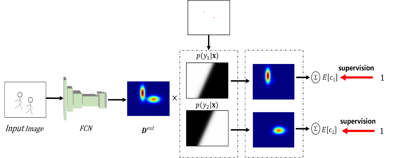
Figure 1. The Bayesian algorithm model
- Motivation
Let  be the density map, where
  represents the 2D pixel location and M is the number of pixels in the density map. Let
  denote the point annotation map for the sample image, where N is the total number of crowds,
  is the starting point location,
  is the corresponding label. The point annotation map contains only one pixel per person (usually the center of the head), is not sparse, and contains no information about object size or shape. It is difficult to directly use such point annotation maps to train a density map estimator. A common remedy for this difficulty is to convert it into a density map of “ground-truth” using the Gaussian kernel.
| 
| (1) |
where  represents the 2D Gaussian distribution evaluated at
  , with the mean at point
  marked, and the isotropic covariance matrix
  .
.
Various recent studies use the above “ground-truth” density map as the learning target and train the density map estimator using the following loss function:
| 
| (2) |
Where  is the distance function and
  is the estimated density map. If a Gaussian kernel of fixed size is adopted
  , it is assumed that all people in the data set have the same head size and shape, which is obviously not true due to the distribution occasional crowds, perspective effects, etc. An alternative is to use an adaptive Gaussian kernel [21] for each
  . Where
  is a distance that depends on the nearest neighbors in the spatial domain, assuming that the crowd is uniformly distributed. Some other methods use specific information such as camera parameters to obtain more accurate perspective maps, but in general such information is not available.
We argue that point annotations in available crowd counting datasets can be considered as weak labels for the density map estimation. It is more reasonable to make annotations instead of learning objectives. Loss functions that impose strict, pixel-to-pixel supervisions in the Eq. (2) on density maps are not always beneficial for enhancing quantity estimation accuracy when used to train the CNN model, because it forces the model to learn incorrect information or even erroneous information.
- The Bayesian Loss
Let x be a random variable representing the spatial position and y be a random variable representing the annotated starting point. Based on the above discussions, instead of converting point annotations into density maps of the “ground-truth” generated by the Equation (1) as the learning objective. The likelihood of  given the label of
  can be proposed as:
| 
| (3) |
To simplify the notation, we ignore the random variables x and y in the following formulas, for example, Eq. (3) becomes  =
=  ). According to the Bayes’s Theorem, given a pixel location
  in a density map, the posterior probability of
  having
  can be calculated as.
| 
| (4) |
In the Eq. (4), the third equality holds when assuming the prior probability  for each class label
  , i.e
, i.e  , without loss of generality. In practice, if we know in advance that crowds are more or less likely to appear in certain places,
  , can be applied.
By using the posterior label probability  and the estimated map density
  , the Bayesian loss can be derived. Let
  denote the amount that
  contributes to
  and
and  be the total relative to
  , the expectation of
  can be expressed as.
| 
| (5) |
Obviously, the number of  ground-truths at each annotation point is one, therefore, the loss function can be expressed as.
| 
| (6) |
where  is the distance function and apply
  distance in the experiments. A special case should be handled when there are no objects in the training images. In such a scenario, the sum of the density map is forced to zero. The proposed loss function is distinct and can be easily applied to a given CNN using a backpropagation training algorithm.
At the inference stage, the posterior label probability  does not have to know in advance, because the estimated density map is aggregated,
  can be eliminated as.
| 
| (7) |
- The Background Pixel Model
For background pixels that are far away from any annotation points, assigning them to any  label is not meaning ful. To better model the background pixels, an additional background label is introduced
  , in addition to the initial labels
  . Therefore, the posterior label probability can be rewritten as.
| 
| (8) |
The final Equation is simplified with the assumption  =
=  , without loss of generality. Similarly, the probability can be re-constructed as.
| 
| (9) |
The expected quantity can be determined for each person and for the entire background as.
| 
| (10) |
| 
| (11) |
In this case, the summation over the entire density map of  includes the number of foregrounds
  and the number of backgrounds
  . Obviously, the background need to count to be zero and the foreground count at each annotation to be one. Hence, the advanced loss function can be expressed as.
| 
| (12) |
Figure 2 Illustration of the geometry of a pseudo-background point, where  represents a pixel in the density map,
  is the nearest start point, and
  is the identified pseudo-background point.
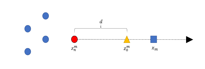
Figure 2. Illustration of the geometry
To determine the background probability, the pseudo background score can be constructed for each pixel according to the following Equation (13).
| 
| (13) |
where  represents the nearest start point of
  and d is a parameter that controls the amplitude between the start point and the pseudo-background points. It can be seen from Figure 2 that the pseudo-background point defined
  , for pixels
  away from the start points. It can be assigned to an alternate background label. The Gaussian kernel is also used to determine the background likelihood as.
| 
| (14) |
- The VGG-19 Model
VGG-19 has 16 convolution layers grouped into 5 blocks. After every block, there is a Maxpool layer that decreases the size of the input image by 2 and increases the number of filters of the convolution layer also by 2. The dimensions of the last three dense layers in block 6 are 4096, 4096, and 1000 respectively. VGG classifies the input images into 1000 different categories. As there are two output classes in this study the dimension of fc8 is set to two. There are other variations of VGG such as VGG-11, VGG-16 and others. VGG-19 has 19.6 billion flops. VGG is a deep CNN used for image classification. The layers in the VGG-19 model are described in Figure 3. It can be briefly as follows:
- The fixed size of RGB (Red-Green-Blue) image (224×224) is given as input to this network, which means the matrix has shape (224, 224, 3).
- The only preprocessing performed is that they subtract the average RGB value from each pixel, which is calculated over the entire training set.
- The kernels used are of size (3×3) with a stride size of 1 pixel, which allows them to cover the entire concept of the image.
- Spatial Padding has been used to preserve the spatial resolution of the image.
- Max Pooling is performed on windows of 2×2 pixels with stride 2.
- This is followed by a rectified linear unit (RELU) to introduce non-linearity to make the classification model better and to improve computation time when previous models used This Tanh or Sigmoid function proved much better than the models.
- Implemented three fully connected layers from which the first two layers have size 4096 and then one layer has 1000 channels for 1000-dimensional ILSVRC classification and the last layer is softmax.
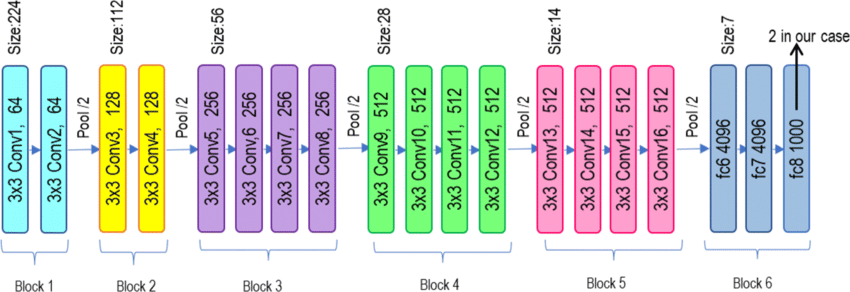
Figure 3. The VGG-19 model architecture
The VGG-19 network is a deep neural network designed to extract features from images. It is called VGG-19 because it has 19 floors (layers) in its architecture. The first layer of VGG-19 is the input layer and the last layer is the output layer, in which the output layer will output the classification probability of objects in the image. Each layer in the VGG-19 network is designed to find different features of the image. The first layers of the VGG-19 network are called convolutional layers. These layers use filters to extract different features of the image. These features can be lines, edges, colors or objects in the image.
The convolutional layers will continue to connect with the activation layers to help the model learn non-linear functions, thereby helping the model be able to find more complex features from the convolutional layers. Then, fully connected layers are used to combine the features extracted by the previous layers. These layers help the model learn classification rules from features in the image. Finally, the output layer will produce the image classification results. In the case of VGG-19, the output layer is a softmax layer, which allows the model to output the classification probabilities of objects in the image. In this paper, we use the pretrained VGG-19 model combined with the Bayesian-loss function to improve accuracy and reduce errors for the problem of estimating the number of crowds.
- RESULTS AND DISCUSSIONS
Based on the theory presented in previous Sections, this Section presents the experimental model and expected results followed by simulation results. Two widely metrics are used for evaluation are the Mean Absolute Error (MAE) and the Mean Squared Error (MSE). MSE and MSE penalize larger errors more, inflating or increasing the mean error value due to the square of the error value. They are defined as.
| 
| (15) |
| 
| (16) |
where K is the number of test images,  and
and  are the number of ground-truths and the number of estimates for
  images, respectively.
- Datasets
Experimental evaluations are performed using four widely used crowd counting benchmark datasets: UCF-QNRF [34], UCF_CC_50 [35], ShanghaiTech [36] part A and part B. Datasets are used for trainning and testing that can be briefly described as follows.
UCF-QNRF [34] is the latest and largest crowd counting dataset consisting of 1.535 images collected from Flickr with 1.25 million point annotations. This is a challenging dataset because it has a wide range of numbers, image resolutions, and lighting conditions. The training set has 1.201 images and the remaining 334 images are used for testing.
ShanghaiTech [36] includes Part A and Part B. In Part A, there are 300 images for training and 182 images for testing. All images are crawled from the internet, and most of them are images of very crowded scenes such as protests and major sporting events. Part B has 400 training images and 316 testing images taken from busy streets in Shanghai. Part A has a significantly higher density than Part B.
UCF_CC_50 [35] contains 50 grayscale images with different resolutions. The average count per image is 1.280, and the minimum and maximum counts are 94 and 4.532, respectively. Since this is a small-scale dataset and does not split the defined data for training and testing, we perform a five-fold cross to get the average testing results. The data set includes images and corresponding annotation files as described in Figure 4.
Figure 4. The data folder structure
- The Trainning Model
We use a standard image classification network backbone, with the final pooling layers and subsequent fully connected layers removed. In the simulation, experiments are conducted by using the VGG-19 network [33]. The output of the backbone is upsampled to 1/8 of the input image size by parallel interpolation, then feed it into regression, which consists of two 3 × 3 convolutional layers with 256 and 128 channels, respectively, and 1 × 1 convolutional layer, to obtain the density map. The regression header is initialized by the MSRA [37] initiator and the backbone is pre-trained on ImageNet. The optimization function with an initial learning rate of 10-5 is used to update the parameters. The network structure is described as shown in Figure 5.
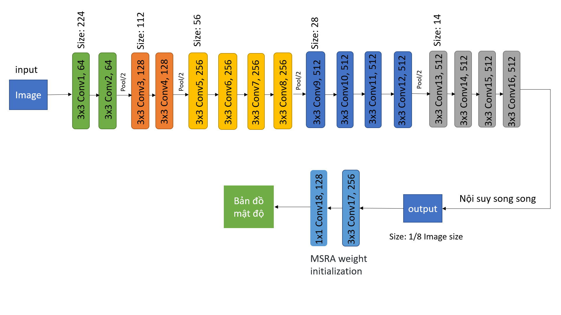


Figure 5. The training network structure
The training data are augmented using random crop and flip. It is noted that image resolution in UCF-QNRF varies widely from 0.08 to 66 megapixels. However, the conventional CNN cannot process images with all types of scales due to its limited receptive field. Therefore, the shorter side of each image is limited to within 2048 pixels in UCF-QNRF. Images are then randomly cropped for training, the crop size of 256 × 256 is used for ShanghaiTechA and UCF_CC_50 where the image resolution is smaller, the size of 512 × 512 is used for ShanghaiTechB and UCF-QNRF. The Gaussian parameter are set in Eq. (3) and Eq. (14) to 8 and the distance parameter d in Eq. (13) to 15% of the shorter side of the image. The parameters are chosen on the evaluation set (120 images randomly sampled from the training set) of UCF-QNRF.
- Experimental Evaluation
We compare the proposed method with baseline and state-of-the-art methods on benchmark datasets described in previous section. For a fair comparison, the base method (Baseline) shares the same network structure (VGG-19) and training procedure as ours using Eq. (2). Specifically, geometric adaptation kernels are applied to UCF-QNRF, ShanghaiTech Part A, and UCF_CC_50, while a fixed Gaussian kernel with σ = 15 is used for ShanghaiTechB. The Bayesian loss (Bayesian) is included in the study. The experimental results are shown in Table 1 and the highlights can be summarized as follows:
Table 1. Results of evaluating MSE, MAE on 4 datasets of the proposed Bayesian algorithm and the Baseline method
Datasets Methods | UCF-QNRF | ShanghaiTech Part A | ShanghaiTech Part B | UCF_CC_50 |
MAE | MSE | MAE | MSE | MAE | MSE | MAE | MSE |
Baseline | 105.6 | 181.5 | 67.8 | 110.1 | 8.4 | 13.6 | 246.5 | 330.5 |
Bayesian | 91.6 | 161.0 | 64.8 | 104.0 | 7.8 | 13.2 | 236.4 | 315.6 |
From Table 1, we can find the followings:
- The proposed Bayesian algorithm gives better results than the other methods.
- Bayesian achieved good accuracy on all four datasets. On the latest and most challenging UCF-QNRF dataset, it reduces the MAE and MSE values of the best method by 40.9 and 28.0, respectively. It is worth mentioning that our method does not use any external detection model or multi-scale structure.
- The Bayesian algorithm significantly outperforms the baseline on all four datasets. The Bayesian performs 15% improvement on UCF-QNRF, 9% on Shanghai, 8% on Shanghai, and 8% on UCF_CC_50, respectively.
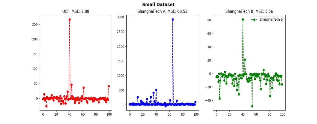
The estimated density is visualized maps using different loss functions during training as shown in Figure 6. From the estimated density results, we can see that the Baseline technique provides results with high errors, whereas the proposed method provides higher accuracy. In the next experiments, the MSE are evaluated the performance on two large and small data sets at σ values, the results are shown in Figure 7 and Figure 8.
From Figure 7 and Figure 8 we can easily see that our Bayesian method works well on small data sets, giving small MSE values. Our method benefits from the proposed probabilistic model that constructs a soft posterior probability if the pixel is close to some starting point. On the other hand, in sparse areas, the Baseline method cannot recognize each person well, while our methods predict more accurate results both in terms of count estimation and localization.
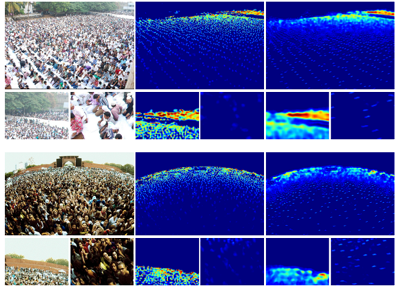
Figure 6. The estimated density map
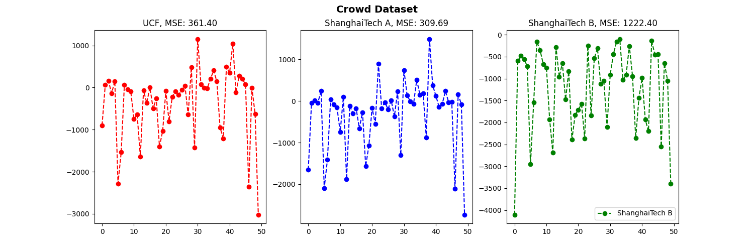
Figure 7. MSE results of the Bayesian method on large data sets at different σ values

Figure 8. MSE results of the Bayesian method on small data sets at different σ values
Cross-dataset evaluation: To further explore the generalizability of different loss functions, we conduct Cross-Dataset experiments with the VGG-19 network. In this experiment, models are trained on one dataset and tested on other models without further fine-tuning. More specifically, we train the models on the largest UCF-QNRF dataset and test them on UCF_CC_50, ShanghaiTechA, and ShanghaiTechB, respectively. As can be seen from Table 2, the method has a certain generalizability and outperforms the Baseline method on all datasets.
Table 2. Results of the cross-dataset evaluation. The models are trained on the UCF-QNRF set and tested on other data sets
Methods | ShanghaiTechA | ShanghaiTechB | UCF_CC_50 |
MAE | MSE | MAE | MSE | MAE | MSE |
Baseline | 72.8 | 128.1 | 17.2 | 29.9 | 322.7 | 557.7 |
Bayeasian | 71.6 | 118.2 | 16.1 | 26.6 | 310.8 | 538.8 |
Limiting the image resolution. We realized that the image resolution of the UCF-QNRF dataset is quite large and wide, the single CNN model cannot handle such a large volume of variables. Therefore, we limit the image resolution to 2048 pixels. As can be seen from Table 3, two methods benefit from rescaling and the Bayesian method outperforms in both settings.
Table 3. Effect of image resolution on UCF-QNRF dataset
Methods | With Resize | Without Resize |
MAE | MSE | MAE | MSE |
Baseline | 105.5 | 182.5 | 128.6 | 191.7 |
Bayeasian | 92.5 | 162.5 | 114.9 | 186.8 |
The proposed loss function can be easily applied to any network structure to improve its performance in the task of crowd size estimation. Here we apply the proposed loss function to both VGG-19 and Alexnet and compare with the basic loss function. The quantitative results from Table 4 indicate that the Bayesian loss function outperforms the baseline loss function significantly on both networks.
Table 4. Performance of models using different backbones on the UCF-QNRF dataset.
Backbones | VGG-19 | AlexNet |
Methods | MAE | MSE | MAE | MSE |
Baseline | 105.6 | 184.2 | 130.5 | 220.8 |
Bayeasian | 92.6 | 164.0 | 121.1 | 202.2 |
- The Crowd Number Warning Application
In addition to performance evaluation, the crowd warning application is also developed. When the crowd exceeds the allowed limit based on the Bayesian proposal method and the PyQt5 framework of the python programming language (Figure 9). The developed crowd estimation application includes the following functions:
- Select video, ip camera or available image.
- Draw the region of interest (ROI) area to estimate the crowd.
- The results of estimating the number of crowds are displayed in the “People estimate”.
Moreover, when the number of crowds exceeds a pre-defined threshold, the application will generates a warning. The application has the function of calculating crowd numbers real-time for future data retrieval.
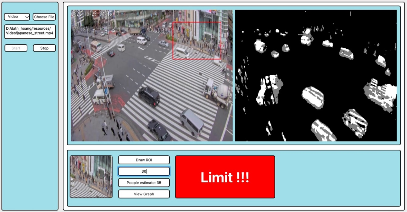
Figure 9. Alarm function if the number of people exceeds the threshold
- CONCLUSIONS
In this paper, the number of crowds can be estimated by using the Bayesian loss function with point monitoring. Different from previous techniques that convert point annotations into ground-truth density maps using a Gaussian kernel with pixel supervision, the loss function applies more reliable supervision using count expectations at each annotated point. Extensive experiments have demonstrated the advantages of the proposed technique in terms of accuracy, robustness, and generalization. The proposed technique showcases a 106.0 reduction in MSE and a 91.6 reduction in MAE over state-of-the-art techniques. The current formulation is quite general then it can easily incorporate other knowledge, e.g. specific foreground or background priors, rates and timing possibilities, and other events to further improve the proposed method.
REFERENCES
- S. A. Velastin, J. H. Yin, A. C. Davies, M. A. Vicencio-Silva, R. E. Allsop, and A. Penn, “Analysis of crowd movements and densities in built-up environments using image processing,” in Proc. IEE Colloquium Image Processing for Transport Applications, 1993, pp. 8/1-8/6, 1993, https://ieeexplore.ieee.org/abstract/document/280223.
- S. A. Velastin, J. H. Yin, A. C. Davies, M. A. Vicencio-Silva, R. E. Allsop and A. Penn, "Automated measurement of crowd density and motion using image processing," Seventh International Conference on Road Traffic Monitoring and Control, 1994., pp. 127-132, 1994, https://doi.org/10.1049/cp:19940440.
- A. N. Marana, L. F. Costa, R. A. Lotufo and S. A. Velastin, "On the efficacy of texture analysis for crowd monitoring," Proceedings SIBGRAPI'98. International Symposium on Computer Graphics, Image Processing, and Vision (Cat. No.98EX237), pp. 354-361, 1998, https://doi.org/10.1109/SIBGRA.1998.722773.
- A. N. Marana et.al., “Automatic estimation of crowd density using texture,” Safety Sci., vol. 28, pp. 165-175, 1998, https://doi.org/10.1016/S0925-7535(97)00081-7.
- R. M. Haralick, “Statistical and structural approaches to texture,” Proc. IEEE, vol. 67, pp. 786-804, 1979, https://doi.org/10.1109/PROC.1979.11328.
- A. N. Marana, L. Da Fontoura Costa, R. A. Lotufo and S. A. Velastin, "Estimating crowd density with Minkowski fractal dimension," 1999 IEEE International Conference on Acoustics, Speech, and Signal Processing. Proceedings. ICASSP99 (Cat. No.99CH36258), vol. 6, pp. 3521-3524, 1999, https://doi.org/10.1109/ICASSP.1999.757602.
- S.-Y. Cho, T. W. S. Chow, and C.-T. Leung, “A neural-based crowd estimation by hybrid global learning algorithm,” IEEE Trans. Syst., Man, Cybern. B, vol. 29, pp. 535-541, 1999, https://doi.org/10.1109/3477.775269.
- H. A. Rowley, S. Baluja, and T. Kanade, “Neural network-based face detection,” IEEE Trans. Pattern Anal. Machine Intell., vol. 20, pp. 23-38, 1998, https://doi.org/10.1109/34.655647.
- M. Oren, C. Papageorgiou, P. Sinha, E. Osuna and T. Poggio, "Pedestrian detection using wavelet templates," Proceedings of IEEE Computer Society Conference on Computer Vision and Pattern Recognition, pp. 193-199, 1997, https://doi.org/10.1109/CVPR.1997.609319.
- O. Chapelle, P. Haffner, and V. N. Vapnik, “Support vector machines for histogram-based image classification,” IEEE Trans. Neural Networks, vol. 10, pp. 1055–1064, Sept. 1999, https://doi.org/10.1109/72.788646.
- J. L. Polus, Schofer, and A. Ushpiz, “Pedestrian flow and level of service,” J. Transp. Eng., vol. 109, pp. 46–56, 1983, https://doi.org/10.1061/(ASCE)0733-947X(1983)109:1(46).
- S.-F. Lin, J.-Y. Chen, and H.-X. Chao, “Estimation of number of people in crowded scenes using perspective transformation,” IEEE Trans. Systems, Man, and Cybernetics, Part A, vol. 31, no. 6, pp. 645-654, 2001, https://doi.org/10.1109/3468.983420.
- M. Li, Z. Zhang, K. Huang, and T. Tan, “Estimating the number of people in crowded scenes by MID based foreground segmentation and head-shoulder detection,” in Proc. International Conference on Pattern Recognition (ICPR), pp. 1-4, 2008, https://doi.org/10.1109/ICPR.2008.4761705.
- W. Ge and Robert T. Collins, “Marked point processes for crowd counting,” in Computer Vision and Pattern Recognition (CVPR), 2009, pp. 2913-2920, 2009, https://doi.org/10.1109/CVPRW.2009.5206621.
- S. Lazebnik, C. Schmid and J. Ponce, "Beyond Bags of Features: Spatial Pyramid Matching for Recognizing Natural Scene Categories," 2006 IEEE Computer Society Conference on Computer Vision and Pattern Recognition (CVPR'06), pp. 2169-2178, 2006, https://doi.org/10.1109/CVPR.2006.68.
- Pedro F Felzenszwalb, David A McAllester, Deva Ramanan, et al., “A discriminatively trained, multiscale, deformable part model,” in Proc. Computer Vision and Pattern Recognition (CVPR), pp. 1-8, 2008, https://doi.org/10.1109/CVPR.2008.4587597.
- A. Krizhevsky, I. Sutskever, and G. E. Hinton, “Imagenet classification with deep convolutional neural networks,” in Advances in Neural Information Processing Systems (NIPS), vol. 25, no. 2, pp. 84-90, 2012, https://doi.org/10.1145/3065386.
- A. B. Chan, Zhang-Sheng John Liang and N. Vasconcelos, "Privacy preserving crowd monitoring: Counting people without people models or tracking," 2008 IEEE Conference on Computer Vision and Pattern Recognition, pp. 1-7, 2008, https://doi.org/10.1109/CVPR.2008.4587569.
- D. Ryan, S. Denman, C. Fookes, and S. Sridharan, “Crowd counting using multiple local features,” In DICTA, 2009, https://doi.org/10.1109/DICTA.2009.22.
- B. Liu and N. Vasconcelos, "Bayesian Model Adaptation for Crowd Counts," 2015 IEEE International Conference on Computer Vision (ICCV), pp. 4175-4183, 2015, https://doi.org/10.1109/ICCV.2015.475.
- H. Idrees, M. Tayyab, K. Athrey, D. Zhang, S. Al-Maadeed, et. al., “Composition loss for counting density map estimation and localization in dense crowds,” in Proc. European Conference on Computer Vision (ECCV), pp. 544-559, 2018, https://doi.org/10.1007/978-3-030-01216-8_33.
- S. Zhang, G. Wu, J. P. Costeira, and J. M. Moura, “FCN-rLSTM: Deep spatio-temporal neural networks for vehicle counting in city cameras,” in Proc. International Conference on Pattern Recognition (ICCV), 2017, pp.3687-3696, 2017, https://doi.org/10.1109/ICCV.2017.396.
- K. Sirinukunwattana, S. E. A. Raza, Y. -W. Tsang, D. R. J. Snead, I. A. Cree and N. M. Rajpoot, "Locality Sensitive Deep Learning for Detection and Classification of Nuclei in Routine Colon Cancer Histology Images," in IEEE Transactions on Medical Imaging, vol. 35, no. 5, pp. 1196-1206, 2016, https://doi.org/10.1109/TMI.2016.2525803.
- X. Liu, J. Weijer, and A. D. Bagdanov, “Leveraging unlabeled data for crowd counting by learning to rank,” in Computer Vision and Pattern Recognition (CVPR), pp. 7661-7669, 2018, https://doi.org/10.1109/CVPR.2018.00799.
- V. Lempitsky and A. Zisserman, “Learning to count objects in images,” in Advances in Neural Information Processing Systems (NIPS), pp. 1324-1332, 2010, https://shorturl.at/BTkkk.
- L. Fiaschi, U. Koethe, R. Nair and F. A. Hamprecht, "Learning to count with regression forest and structured labels," Proceedings of the 21st International Conference on Pattern Recognition (ICPR2012), pp. 2685-2688, 2012, https://ieeexplore.ieee.org/abstract/document/6460719.
- V.-Q. Pham, T. Kozakaya, O. Yamaguchi, and R. Okada, “COUNT forest: Co-voting uncertain number of targets using random forest for crowd density estimation,” in Proc. International Conference on Pattern Recognition (ICCV), pp. 3253-3261, 2015, https://doi.org/10.1109/ICCV.2015.372.
- Z. Shi, L. Zhang, Y. Liu, X. Cao, Y. Ye, M. M. Cheng, and G. Zheng, “Crowd counting with deep negative correlation learning,” in Proc. Computer Vision and Pattern Recognition (CVPR), pp. 5382-5390, 2018, https://doi.org/10.1109/CVPR.2018.00564.
- L. Liu, H. Wang, G. Li, W. Ouyang, and L. Lin, “Crowd counting using deep recurrent spatial-aware network,” arXiv preprint arXiv:1807.00601, 2018, https://doi.org/10.48550/arXiv.1807.00601.
- X. Cao, Z. Wang, Y. Zhao, and F. Su, “Scale aggregation network for accurate and efficient crowd counting,” in European Conference on Computer Vision (ECCV), pp. 757-773, 2018, https://doi.org/10.1007/978-3-030-01228-1_45.
- V. Ranjan, H. Le, and M. Hoai, “Iterative crowd counting,” in European Conference on Computer Vision (ECCV), pp. 270-285, 2018, https://doi.org/10.1007/978-3-030-01234-2_17.
- C. Zhang, H. Li, X. Wang, and X. Yang, “Cross-scene crowd counting via deep convolutional neural networks,” in Computer Vision and Pattern Recognition (CVPR), pp. 833-841, 2015, https://doi.org/10.1109/CVPR.2016.70.
- K. Simonyan and A. Zisserman, “Very deep convolutional networks for large-scale image recognition,” arXiv preprint arXiv:1409.1556, 2014, https://doi.org/10.48550/arXiv.1409.1556.
- H. Idrees, I. Saleemi, C. Seibert, and M. Shah, “Multi-source multi-scale counting in extremely dense crowd images,” in Proc. Computer Vision and Pattern Recognition (CVPR), pp. 730-734, 2013, https://doi.org/10.1109/CVPR.2013.329.
- Y. Zhang, D. Zhou, S. Chen, S. Gao, and Y. Ma, “Single-image crowd counting via multi-column convolutional neural network,” in Proc. Computer Vision and Pattern Recognition (CVPR), pp. 589-597, 2016, https://doi.org/10.1109/CVPR.2016.70.
- H. Idrees, M. Tayyab, K. Athrey, D. Zhang, S.Al-Maadeed, N. Rajpoot, and M. Shah, “Composition loss for counting density map estimation and localization in dense crowds,” in European Conference on Computer Vision (ECCV), pp. 544–559, 2018, https://doi.org/10.1007/978-3-030-01216-8_33.
- K. He, X. Zhang, S. Ren, and J. Sun, “Delving deep into rectifiers: Surpassing human-level performance on imagenet classification,” in International Conference on Pattern Recognition (ICCV), pp. 1026-1034, 2015, https://doi.org/10.1109/ICCV.2015.123.
AUTHOR BIOGRAPHY

| Ha Duyen Trung studied Engineer in Electronics and Telecommunications from Hanoi University of Science and Technology (HUST), Hanoi, Vietnam from 1998 to 2003, master and PhD in Communications Engineering from Chulalongkorn University, Bangkok, Thailand from 2003 to 2009, respectively. From 2007 to 2008, he was a research student at the Mobile Communications Laboratory (Araki Lab), Tokyo Institute of Technology, Japan. In 2012, Dr. Trung spent three months as a visiting scholar at Aizu University, Japan. He has been a lecturer at HUST since 2009. He joined HEEAP University Faculty Development Training at Arizona State University, AZ, USA in 2015. He published various research papers in the areas of image signal processing, IoT platform and related technologies, optical wireless communications, signal processing for the next mobile communications, UAV communications, satellite-based positioning, and navigation, and so on. |
Estimation of Crowd Density Using Image Processing Techniques with Background Pixel Model and Visual Geometry Group (Ha Duyen Trung)